
01. 30-Day Fed Funds Futures (ZQ) Data from Databento#
The CME’s 30-Day Fed Funds futures (product code ZQ) are the raw material behind the famous CME FedWatch tool. Each monthly contract settles at
where \(\bar{r}\) is the calendar-day average of the daily effective federal funds rate (EFFR) over the contract month, as published by the New York Fed. Days without a published rate (weekends, holidays) carry forward the previous day’s rate.
That settlement rule is what makes ZQ prices interesting: buying the September contract at 96.30 is a bet that fed funds will average \(100 - 96.30 = 3.70\%\) during September. The price is the market’s forecast of Fed policy for that month. In the next notebook we turn these prices into FedWatch-style probabilities for the next FOMC decision; here we get to know the data itself.
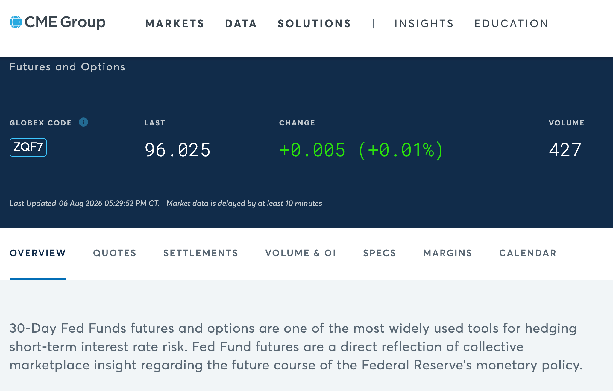
CME’s product page
for 30-Day Fed Funds futures — here quoting ZQF7, a symbol we will learn
to decode below.
How the data was pulled#
This project follows the course convention: pull_* scripts hit the network
and cache to _data/; notebooks only ever load_* from that cache, so they
run offline. The pull lives in pull_fed_funds_futures.py and its core is
just this (shown here, not executed):
import databento as db

client = db.Historical(key=DATABENTO_API_KEY)

query = dict(
    dataset="GLBX.MDP3",  # CME Globex market data
    symbols=["ZQ.FUT"],   # parent symbology: every listed ZQ contract at once
    stype_in="parent",
    schema="ohlcv-1d",    # one OHLCV bar per contract per trading day
    start=START_DATE,     # trailing ~6 months
    end=END_DATE,
)

cost = client.metadata.get_cost(**query)  # free metadata call
assert_within_budget(cost)                # abort BEFORE any paid call

df = client.timeseries.get_range(**query).to_df()
Things worth noticing:
Dataset
GLBX.MDP3is CME Globex’s market-by-order feed; Databento derives all simpler schemas from it. Our course subscription is historical-only (no live streaming), and history lags real time by about a day.Parent symbology (
ZQ.FUT) asks for all listed ZQ contracts in one query — outright monthly contracts plus calendar spreads — instead of naming each contract.Schema
ohlcv-1dgives daily open/high/low/close/volume bars, the coarsest (and cheapest) view of the data. The same query withschema="trades"would return every individual trade.The cost guard.
metadata.get_costprices a query for free before we commit to it. This pull costs pennies (it shows $0.00 under the course subscription), but the guard is a habit worth keeping: the same code pointed at a tick-level schema could cost real money.
The cached file is a target of the doit pipeline. To refresh it with the
latest prices, run doit forget pull && doit.
import matplotlib.pyplot as plt
import pandas as pd

import fedwatch
import pull_fed_funds_futures

df = pull_fed_funds_futures.load_fed_funds_futures()
df.head()
| date | symbol | open | high | low | close | volume | |
|---|---|---|---|---|---|---|---|
| 0 | 2026-02-08 | ZQJ6-ZQX6 | -44.0 | -44.0 | -44.0 | -44.0 | 3 |
| 1 | 2026-02-08 | ZQ:BF J6-K6-M6 | 1.5 | 1.5 | 1.5 | 1.5 | 2 |
| 2 | 2026-02-08 | ZQU6-ZQZ6 | -16.0 | -15.5 | -16.0 | -16.0 | 11 |
| 3 | 2026-02-08 | ZQH6-ZQU6 | -34.0 | -34.0 | -34.0 | -34.0 | 3 |
| 4 | 2026-02-08 | ZQN6-ZQU6 | -13.5 | -13.5 | -13.5 | -13.5 | 4 |
Reading the columns and the symbols#
date— the trading date of the bar (Databento stamps daily bars at 00:00 UTC; the pull converts that to a plain date).symbol— the specific contract the bar belongs to.open/high/low/close— prices in index points (100 minus rate).volume— contracts traded that day.
A CME futures symbol has three parts: root + month code + year digit. The month codes are a piece of exchange-floor history worth memorizing:
Code |
F |
G |
H |
J |
K |
M |
N |
Q |
U |
V |
X |
Z |
|---|---|---|---|---|---|---|---|---|---|---|---|---|
Month |
Jan |
Feb |
Mar |
Apr |
May |
Jun |
Jul |
Aug |
Sep |
Oct |
Nov |
Dec |
So ZQU6 = ZQ + U (September) + 6 — the September 2026 contract. Note
the single year digit is ambiguous: ZQU6 could just as well be 2016 or
2036. fedwatch.parse_zq_contract_month resolves it to the unique matching
year near the date of the data, which is safe because ZQ only lists about
three years of contracts at a time.
The parent-symbology pull also returns calendar spreads like
ZQU6-ZQZ6 (buy September, sell December as a package). We don’t need them,
so fedwatch.filter_outright_contracts keeps only symbols matching the
outright pattern.
df["symbol"].nunique(), sorted(df["symbol"].unique())[:12]
(204,
 ['ZQ:BF F7-G7-H7',
  'ZQ:BF F7-G7-J7',
  'ZQ:BF G6-H6-J6',
  'ZQ:BF G6-J6-K6',
  'ZQ:BF G7-H7-J7',
  'ZQ:BF G7-J7-K7',
  'ZQ:BF H6-J6-K6',
  'ZQ:BF H7-J7-K7',
  'ZQ:BF J6-K6-M6',
  'ZQ:BF J6-K6-N6',
  'ZQ:BF J7-K7-M7',
  'ZQ:BF J7-K7-N7'])
df_out = fedwatch.filter_outright_contracts(df).copy()
as_of = df_out["date"].max()
df_out["contract_month"] = pd.PeriodIndex(
    [fedwatch.parse_zq_contract_month(s, as_of) for s in df_out["symbol"]],
    freq="M",
)
df_out.head()
| date | symbol | open | high | low | close | volume | contract_month | |
|---|---|---|---|---|---|---|---|---|
| 7 | 2026-02-08 | ZQG7 | 96.900 | 96.9150 | 96.890 | 96.9150 | 18 | 2027-02 |
| 8 | 2026-02-08 | ZQX6 | 96.845 | 96.8600 | 96.835 | 96.8600 | 149 | 2026-11 |
| 9 | 2026-02-08 | ZQG6 | 96.360 | 96.3625 | 96.360 | 96.3625 | 31 | 2026-02 |
| 11 | 2026-02-08 | ZQM6 | 96.510 | 96.5150 | 96.505 | 96.5150 | 299 | 2026-06 |
| 13 | 2026-02-08 | ZQQ6 | 96.690 | 96.6900 | 96.665 | 96.6850 | 422 | 2026-08 |
Prices as implied rates#
The settlement rule makes translation trivial: implied average rate =
100 − price. One practical wrinkle: contract months far in the future
trade thinly, so a contract may have no bar at all on a given day.
fedwatch.latest_prices_by_contract therefore takes each contract’s last
available close on or before the as-of date rather than insisting on
today’s bar.
latest = fedwatch.latest_prices_by_contract(df)
latest["implied_rate"] = fedwatch.implied_rate(latest["close"])
latest
| symbol | contract_month | date | close | implied_rate | |
|---|---|---|---|---|---|
| 0 | ZQG6 | 2026-02 | 2026-02-27 | 96.3600 | 3.6400 |
| 1 | ZQH6 | 2026-03 | 2026-03-31 | 96.3600 | 3.6400 |
| 2 | ZQJ6 | 2026-04 | 2026-04-30 | 96.3600 | 3.6400 |
| 3 | ZQK6 | 2026-05 | 2026-05-29 | 96.3725 | 3.6275 |
| 4 | ZQM6 | 2026-06 | 2026-06-30 | 96.3750 | 3.6250 |
| 5 | ZQN6 | 2026-07 | 2026-07-31 | 96.3725 | 3.6275 |
| 6 | ZQQ6 | 2026-08 | 2026-08-05 | 96.3675 | 3.6325 |
| 7 | ZQU6 | 2026-09 | 2026-08-05 | 96.3000 | 3.7000 |
| 8 | ZQV6 | 2026-10 | 2026-08-05 | 96.2250 | 3.7750 |
| 9 | ZQX6 | 2026-11 | 2026-08-05 | 96.1700 | 3.8300 |
| 10 | ZQZ6 | 2026-12 | 2026-08-05 | 96.0900 | 3.9100 |
| 11 | ZQF7 | 2027-01 | 2026-08-05 | 96.0600 | 3.9400 |
| 12 | ZQG7 | 2027-02 | 2026-08-05 | 96.0350 | 3.9650 |
| 13 | ZQH7 | 2027-03 | 2026-08-05 | 96.0100 | 3.9900 |
| 14 | ZQJ7 | 2027-04 | 2026-08-05 | 95.9750 | 4.0250 |
| 15 | ZQK7 | 2027-05 | 2026-08-05 | 95.9650 | 4.0350 |
| 16 | ZQM7 | 2027-06 | 2026-08-05 | 95.9550 | 4.0450 |
| 17 | ZQN7 | 2027-07 | 2026-08-05 | 95.9550 | 4.0450 |
| 18 | ZQQ7 | 2027-08 | 2026-08-05 | 95.9650 | 4.0350 |
| 19 | ZQU7 | 2027-09 | 2026-08-05 | 95.9750 | 4.0250 |
| 20 | ZQV7 | 2027-10 | 2026-08-05 | 95.9850 | 4.0150 |
| 21 | ZQX7 | 2027-11 | 2026-08-05 | 96.0100 | 3.9900 |
| 22 | ZQZ7 | 2027-12 | 2026-07-23 | 95.9000 | 4.1000 |
Two pictures of the data#
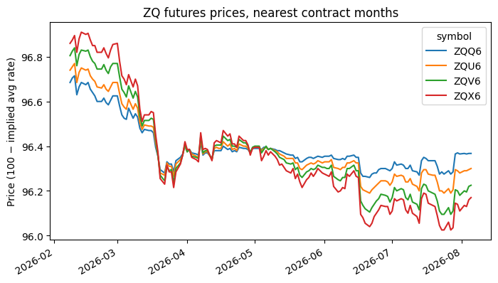
First, the price history of the nearest few contracts over our pull window. Prices drift as the market updates its view of where the Fed is heading — each line is a rolling referendum on one month’s average fed funds rate.
front_symbols = latest.loc[
    latest["contract_month"] >= pd.Period(as_of, freq="M"), "symbol"
].head(4)
prices = df_out[df_out["symbol"].isin(front_symbols)].pivot_table(
    index="date", columns="symbol", values="close"
)
ax = prices.plot(figsize=(8, 4.5))
ax.set_title("ZQ futures prices, nearest contract months")
ax.set_ylabel("Price (100 − implied avg rate)")
ax.set_xlabel("")
plt.show()
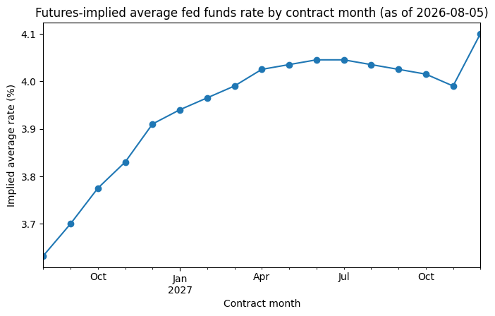
Second, the cross-section on the latest date: the implied average rate for each upcoming contract month. This curve is the market’s forecast of the fed funds path — every step down (up) the market prices in is a future cut (hike). FedWatch is essentially a careful reading of this curve around FOMC meeting dates.
path = latest[latest["contract_month"] >= pd.Period(as_of, freq="M")].copy()
path["month"] = path["contract_month"].dt.to_timestamp()
ax = path.plot(x="month", y="implied_rate", marker="o", legend=False, figsize=(8, 4.5))
ax.set_title(f"Futures-implied average fed funds rate by contract month (as of {as_of.date()})")
ax.set_ylabel("Implied average rate (%)")
ax.set_xlabel("Contract month")
plt.show()
Summary#
ZQ futures settle at 100 minus the monthly average EFFR, so prices map directly to market-expected policy rates.
Databento’s parent symbology +
ohlcv-1dschema deliver every contract’s daily bars in one cheap, cost-guarded query.Symbols encode contract months (root + month code + year digit); spreads get filtered out, thin months use the last available close.
Exercises
Re-run
latest_prices_by_contractwithas_ofset three months back. How did the implied rate path shift?Change the pull’s schema to
ohlcv-1min a scratch script and estimate the cost withmetadata.get_cost(don’t pull!). How much more expensive is minute-level data?Look up today’s front-month contract volume. Why is it so much higher than the volume 18 months out?