Cleaning TRACE Corporate Bond Data: A Walkthrough

Cleaning TRACE Corporate Bond Data: A Walkthrough#

This notebook walks through an end-to-end pipeline for cleaning FINRA TRACE corporate bond transaction data. We start from raw intraday trade reports and progress through filtering, error correction, and daily aggregation to produce an enriched panel with duration, convexity, and credit spreads.

We use a January–February 2024 sample window throughout. The same pipeline runs identically on the full 2002–present history.

import os
import sys
from pathlib import Path

# Ensure src/ is importable regardless of where the notebook executes from.
# When run via dodo.py the cwd is the project root; when run from _output/
# we walk up to find the src/ directory.
_cwd = Path.cwd()
_candidates = [_cwd / "src", _cwd.parent / "src", _cwd]
for _p in _candidates:
    if (_p / "settings.py").exists():
        sys.path.insert(0, str(_p))
        os.chdir(_p.parent)  # set project root as cwd
        break

import matplotlib.pyplot as plt
import matplotlib.dates as mdates
import numpy as np
import polars as pl

from settings import config

DATA_DIR = Path(config("DATA_DIR"))
PULL_DIR = DATA_DIR / "pulled"

plt.rcParams.update({
    "figure.figsize": (10, 4),
    "axes.titlesize": 13,
    "axes.labelsize": 11,
    "figure.dpi": 120,
})

1. What Is TRACE and Why Does Cleaning Matter?#

TRACE (Trade Reporting and Compliance Engine) is operated by FINRA. Every over-the-counter (OTC) corporate bond trade in the United States must be reported to TRACE within 15 minutes of execution. TRACE Enhanced, available from July 2002, provides the most complete data: counterparty identifiers, the full trade lifecycle (original reports, corrections, cancellations, reversals), and both price and volume.

What securities does TRACE cover?#

While this project focuses on corporate bonds, TRACE covers several categories of fixed-income securities:

Corporate bonds (investment-grade, high-yield, and convertible debt)—reported since TRACE launched in July 2002. This is the asset class we work with here.
Agency debentures—reported since March 2010.
Mortgage-backed securities (MBS) and asset-backed securities (ABS), including TBA transactions—reported since May 2011; public dissemination was phased in through 2015.
U.S. Treasury securities—reported since July 2017, but transaction-level public dissemination only began in March 2024, limited to on-the-run nominal coupons on an end-of-day basis. Full Treasury transaction data is not available to the public or researchers.
Rule 144A private placements—reported separately; included in our pipeline via the TRACE 144A feed.

What information is in the public data?#

The corporate bond transaction data that FINRA makes available to the public and to academics includes trade-level details (price, yield, volume, execution time, buy/sell indicator, counterparty type), but dealer identity is either removed or masked. The TRACE Enhanced data available on WRDS does not contain unmasked dealer identifiers.

Data access#

WRDS is the most common academic access point for corporate bond TRACE data (Enhanced, Standard, and 144A feeds). WRDS does not host agency, MBS/ABS, or Treasury TRACE data.
FINRA also makes corporate bond TRACE data available directly to academic institutions and to the public (with delays). MBS/ABS historical data requires a separate agreement with FINRA. Free next-day transaction data and aggregate reports are available on FINRA’s website for non-commercial use.

Unlike equities, which trade on centralized exchanges with a consolidated limit order book, corporate bonds trade OTC through dealer intermediaries. This creates fundamental data-quality challenges:

No consolidated best bid/offer. Prices reflect individually negotiated trades between dealers and customers or between dealers.
Market microstructure noise (MMN) is substantially larger than in equities. Transaction prices contain bid-ask bounce and dealer markups.
Trade lifecycle records. A single economic trade can generate multiple TRACE records (original report, cancellation, correction, reversal).

Using uncleaned TRACE data leads to biased return estimates and spurious factor premia—a problem documented extensively in recent research.

Why this pipeline exists: lessons from the literature#

Dickerson, Robotti, and Rossetti (2024), “Common pitfalls in the evaluation of corporate bond strategies” (SSRN 4575879):

Large abnormal returns documented for many corporate bond strategies are primarily artifacts of (a) ignoring market microstructure noise in transaction-based prices and (b) applying ex-post (asymmetric) data filtering.
MMN magnitude: The short-term reversal premium drops from 0.90% per month to approximately zero after correcting for MMN. Price-based signals (credit spread, yield) show 50–65% reductions in return premiums.
Ex-post filtering bias: Out of 480 ex-ante filtered strategies, only 2 (0.4%) produce significant momentum premia. With ex-post filtering, that number jumps to 119 (25%)—almost entirely an artifact.
Recommendation: Use an “implementation gap” (source signal prices at least one day before month-end execution prices) and apply only ex-ante filters with information available at portfolio formation.

Dickerson, Robotti, and Rossetti (2026), “The Corporate Bond Factor Replication Crisis”:

Evaluates 108 signals across 9 thematic clusters using the Open Bond Asset Pricing (OBAP) framework.
Two sources systematically inflate reported premia: (a) OTC microstructure that prevents execution at signal-formation prices, and (b) ex-post filtering that embeds future information into portfolio construction.
Result: The majority of previously documented anomalies fail—they are artifacts of measurement error, not genuine risk premia.
Provides an open-source end-to-end TRACE data pipeline (the basis for the Stage 0 cleaning code in this project).

Pipeline overview#

Raw TRACE Enhanced   --[FISD filter]-->   FISD-filtered   --[11 filters + daily agg]-->   Stage 0
  (intraday trades)                       (standard US                                     (daily panel)
                                           corporate bonds)                                    |
                                                                                               v
                                                             Stage 1  <--[QuantLib + ratings + linker]
                                                        (enriched panel: duration, convexity,
                                                         credit spreads, ratings, equity IDs)

2. Data Sources and Pipeline Overview#

The pipeline consumes 14 datasets from four providers: WRDS (TRACE trade feeds and FISD bond reference tables), the Liu-Wu yield curve (Google Sheets), the Kenneth French Data Library (Dartmouth), and the Open Source Bond Asset Pricing project (openbondassetpricing.com). These fall into three groups: trade data (the raw transactions we clean), bond reference data (characteristics, ratings, and identifiers we merge in), and validation / linkage data (external benchmarks and cross-asset links).

#	Dataset	Source	Pipeline role	Stage
1	TRACE Enhanced	WRDS	Primary trade data (Jul 2002–Sep 2024)	Pull $\to$ FISD filter $\to$ Stage 0 $\to$ Stage 1
2	TRACE Standard	WRDS	Extends trade coverage (Oct 2024+)	Pull $\to$ FISD filter $\to$ Stage 0 $\to$ Stage 1
3	TRACE 144A	WRDS	Private-placement trades (Rule 144A)	Pull $\to$ FISD filter $\to$ Stage 0 $\to$ Stage 1
4	FISD Issue	WRDS	Bond-level reference (coupon, maturity, offering)	Pre-processing + Stage 1
5	FISD Issuer	WRDS	Issuer attributes (SIC code, country)	Pre-processing
6	FISD Amount Outstanding	WRDS	Time-varying par amount outstanding	Stage 1
7	FISD Ratings (S&P)	WRDS	Historical S&P credit ratings	Stage 1
8	FISD Ratings (Moody’s)	WRDS	Historical Moody’s credit ratings	Stage 1
9	FISD Redemption	WRDS	Callable-bond flag	Stage 1
10	Liu-Wu Treasury Yields	Google Sheets	Zero-coupon yield curve for credit spreads	Stage 1
11	Fama-French SIC Codes	Dartmouth	Industry classification (FF-17 / FF-30)	Stage 1
12	OSBAP Linker (Fang, 2025)	OSBAP	Bond-to-equity identifier mapping	Stage 1
13	OSBAP Corporate Bond Returns	OSBAP	Validation benchmark (duration, spreads)	Testing only
14	OSBAP Treasury Bond Returns	OSBAP	Not currently consumed	—

Three TRACE feeds#

FINRA publishes corporate bond trades through three separate reporting channels. The pipeline pulls all three and merges them after cleaning:

Enhanced is the workhorse dataset. It has the longest history (July 2002 onward), the richest columns (exact volume in entrd_vol_qt, counterparty IDs in cntra_mp_id), and is the target of most academic TRACE-cleaning papers.
Standard is the real-time public feed. WRDS makes it available from October 2024, so it extends coverage into months where Enhanced is not yet released. It uses a slightly different column schema (ascii_rptd_vol_tx for volume, side instead of rpt_side_cd).
144A captures a separate market segment: bonds sold to qualified institutional buyers under SEC Rule 144A. These private placements do not appear in the Enhanced or Standard feeds.

When the three are combined in Stage 1, Enhanced takes priority. Standard is clipped to dates after the Enhanced maximum date to avoid overlap, while 144A rows are kept unconditionally (they cover distinct bonds). Duplicate (cusip, date) pairs across feeds are resolved with preference Enhanced > Standard > 144A.

FISD reference data (6 files)#

The Mergent Fixed Income Securities Database (FISD), accessed via WRDS, provides the bond-level reference data that the pipeline relies on throughout:

FISD Issue — One row per bond. Coupon, maturity, offering date, offering amount, bond type, currency, and other characteristics. Combined with FISD Issuer to build the FISD universe of standard US corporate bonds (10 screens: USD only, fixed-rate, non-convertible, non-ABS, etc.). Also used in Stage 1 to map issue_id to CUSIP for ratings and amount-outstanding merges.
FISD Issuer — One row per issuer. Provides the SIC code (used for Fama-French industry classification) and country of domicile.
FISD Amount Outstanding History — Time-varying par amount. Merged into the Stage 1 panel via merge_asof (backward on date) so each bond-day observation reflects the most recent outstanding amount.
FISD Ratings (S&P) and FISD Ratings (Moody’s) — Historical credit ratings (one row per rating event). Converted to numeric scales in Stage 1 and merged via merge_asof so each bond-day gets the most recent rating. A composite rating is computed as the average of the S&P and Moody’s numeric scores.
FISD Redemption — Callable/redeemable flags. Produces a binary callable indicator merged into Stage 1.

Liu-Wu Treasury yields#

The Liu-Wu zero-coupon Treasury yield curve (sourced from a Google Sheets mirror of the original Liu-Wu dataset) provides daily yields at 1, 2, 5, 7, 10, 20, and 30-year maturities. Stage 1 interpolates this curve at each bond’s remaining maturity and subtracts the duration-matched Treasury yield from the bond’s yield-to-maturity to compute the credit spread.

Fama-French SIC codes#

The Kenneth French Data Library provides mappings from SIC code ranges to the Fama-French 17-industry and 30-industry classification systems. In Stage 1, each bond issuer’s SIC code (from FISD Issuer) is matched to these ranges, adding ff17num and ff30num industry identifiers to every bond-day observation.

Open Source Bond Asset Pricing (OSBAP) datasets#

The OSBAP project at openbondassetpricing.com provides three files that play different roles:

OSBAP Linker (Fang, 2025) — A core Stage 1 input. Maps issuer CUSIPs (first 6 characters) to equity identifiers (PERMNO, PERMCO, GVKEY) over time. Many bonds are issued through subsidiaries that do not share the parent’s identifiers, and 19% of CUSIP-6s change ultimate parents during the sample. The linker resolves this using CUSIP-ticker mappings from ICE and TRACE, the ticker-GVKEY mapping from Compustat, and the CRSP-Compustat link, with extensive hand corrections. Forward-filled and left-joined on (issuer CUSIP, year-month) in Stage 1 Step 7.
OSBAP Corporate Bond Returns — A validation-only benchmark. The test suite (test_stage1_vs_open_source.py) aggregates Stage 1 daily output to month-end, inner-joins with OSBAP on (cusip, date), and checks that yield-to-maturity, modified duration, convexity, credit spread, time-to-maturity, bond market cap, bond age, and industry classifications are highly correlated and within acceptable tolerance. This is how we confirm the pipeline is producing correct results.
OSBAP Treasury Bond Returns — Pulled for completeness but not currently consumed by any processing or validation stage.

3. Raw TRACE Enhanced Data#

Each row in raw TRACE is a single trade report. Key columns:

Column	Description
`cusip_id`	9-character bond identifier
`trd_exctn_dt` / `trd_exctn_tm`	Execution date and time
`rptd_pr`	Reported price per $100 par
`entrd_vol_qt`	Par volume traded
`yld_pt`	Yield at time of trade
`trc_st`	Status code: T = original trade, X = cancellation, C = correction, W/Y = reversal
`rpt_side_cd`	B = buy, S = sell (from reporting dealer perspective)
`cntra_mp_id`	Counterparty: C = customer, D = inter-dealer
`msg_seq_nb` / `orig_msg_seq_nb`	Sequence numbers for matching corrections to originals

raw = pl.scan_parquet(
    PULL_DIR / "trace_enhanced" / "**/*.parquet",
    hive_partitioning=True,
    missing_columns="insert",
).filter(pl.col("year") == 2024, pl.col("month") == 1)

n_raw = raw.select(pl.len()).collect().item()
cols_raw = raw.collect_schema().names()
print(f"Raw TRACE Enhanced (Jan 2024) -- Rows: {n_raw:,}  |  Columns: {len(cols_raw)}")

Raw TRACE Enhanced (Jan 2024) -- Rows: 3,768,457  |  Columns: 21

Example rows#

raw.head(10).collect()

shape: (10, 21)

cusip_id	bond_sym_id	trd_exctn_dt	trd_exctn_tm	days_to_sttl_ct	lckd_in_ind	wis_fl	sale_cndtn_cd	msg_seq_nb	trc_st	trd_rpt_dt	trd_rpt_tm	entrd_vol_qt	rptd_pr	yld_pt	asof_cd	orig_msg_seq_nb	rpt_side_cd	cntra_mp_id	year	month
str	str	date	i64	str	str	str	str	str	str	date	i64	f64	f64	f64	str	str	str	str	i64	i64
"02209SBD4"	"MO4797929"	2024-01-01	78261000000000	null	null	"N"	null	"0000453"	"T"	2024-01-02	28812000000000	3000.0	100.049	4.787982	"A"	null	"B"	"D"	2024	1
"02209SBD4"	"MO4797929"	2024-01-01	78261000000000	null	null	"N"	null	"0000555"	"T"	2024-01-02	28813000000000	3000.0	100.049	4.787982	"A"	null	"S"	"D"	2024	1
"254687FS0"	"DIS4969022"	2024-01-01	81521000000000	null	null	"N"	null	"0000479"	"T"	2024-01-02	28812000000000	5000.0	97.448	4.872966	"A"	null	"B"	"D"	2024	1
"254687FS0"	"DIS4969022"	2024-01-01	81521000000000	null	null	"N"	null	"0000547"	"T"	2024-01-02	28813000000000	5000.0	97.448	4.872966	"A"	null	"S"	"D"	2024	1
"30303M8J4"	"FB5522214"	2024-01-01	81331000000000	null	null	"N"	null	"0000474"	"T"	2024-01-02	28812000000000	10000.0	92.531	4.940009	"A"	null	"B"	"D"	2024	1
"30303M8J4"	"FB5522214"	2024-01-01	81331000000000	null	null	"N"	null	"0000558"	"T"	2024-01-02	28813000000000	10000.0	92.531	4.940009	"A"	null	"S"	"D"	2024	1
"404280DH9"	"HBC5458071"	2024-01-01	81225000000000	null	null	"N"	null	"0000072"	"T"	2024-01-02	28807000000000	2e6	101.0	null	"A"	null	"S"	"A"	2024	1
"458140BX7"	"INTC5238071"	2024-01-01	81367000000000	null	null	"N"	null	"0000477"	"T"	2024-01-02	28812000000000	10000.0	69.707	4.993	"A"	null	"B"	"D"	2024	1
"458140BX7"	"INTC5238071"	2024-01-01	81367000000000	null	null	"N"	null	"0000566"	"T"	2024-01-02	28813000000000	10000.0	69.707	4.993	"A"	null	"S"	"D"	2024	1
"46647PCQ7"	"JPM5260072"	2024-01-01	76026000000000	null	null	"N"	null	"0000676"	"T"	2024-01-02	28814000000000	3e6	98.89	null	"A"	null	"B"	"A"	2024	1

raw.tail(10).collect().glimpse()

Rows: 10
Columns: 21
$ cusip_id         <str> 'Y8085FBU3', 'Y8085FBU3', 'Y8085FBU3', 'Y8846QAG1', 'Y8846QAG1', 'Y8846QAG1', 'Y8846QAG1', 'Y8850AAB0', 'Y93541AA1', 'Y93541AA1'
$ bond_sym_id      <str> 'HXSCF5730863', 'HXSCF5730863', 'HXSCF5730863', 'PTFRF4937561', 'PTFRF4937561', 'PTFRF4937561', 'PTFRF4937561', 'TNABY4760205', 'CHVKF4590832', 'CHVKF4590832'
$ trd_exctn_dt    <date> 2024-01-31, 2024-01-31, 2024-01-31, 2024-01-31, 2024-01-31, 2024-01-31, 2024-01-31, 2024-01-31, 2024-01-31, 2024-01-31
$ trd_exctn_tm     <i64> 36763000000000, 36763000000000, 42120000000000, 6279000000000, 6279000000000, 8933000000000, 30235000000000, 42808000000000, 16600000000000, 16600000000000
$ days_to_sttl_ct  <str> null, null, null, null, null, null, null, null, null, null
$ lckd_in_ind      <str> null, null, null, null, null, null, null, null, null, null
$ wis_fl           <str> 'N', 'N', 'N', 'N', 'N', 'N', 'N', 'N', 'N', 'N'
$ sale_cndtn_cd    <str> null, null, null, null, null, null, null, null, null, null
$ msg_seq_nb       <str> '0040572', '0040573', '0087790', '0001307', '0001333', '0002973', '0007559', '0093183', '0004037', '0004038'
$ trc_st           <str> 'T', 'T', 'T', 'T', 'T', 'T', 'T', 'T', 'T', 'T'
$ trd_rpt_dt      <date> 2024-01-31, 2024-01-31, 2024-01-31, 2024-01-31, 2024-01-31, 2024-01-31, 2024-01-31, 2024-01-31, 2024-01-31, 2024-01-31
$ trd_rpt_tm       <i64> 36766000000000, 36766000000000, 42245000000000, 28817000000000, 28817000000000, 28855000000000, 30236000000000, 42838000000000, 28890000000000, 28890000000000
$ entrd_vol_qt     <f64> 200000.0, 200000.0, 400000.0, 1600000.0, 1600000.0, 200000.0, 1000000.0, 210000.0, 1000000.0, 1000000.0
$ rptd_pr          <f64> 101.11, 101.11, 101.153, 98.625, 98.625, 98.63, 98.55, 99.911, 63.875, 63.875
$ yld_pt           <f64> null, null, null, null, null, null, null, null, null, null
$ asof_cd          <str> null, null, null, null, null, null, null, null, null, null
$ orig_msg_seq_nb  <str> null, null, null, null, null, null, null, null, null, null
$ rpt_side_cd      <str> 'S', 'B', 'S', 'S', 'B', 'B', 'B', 'B', 'S', 'B'
$ cntra_mp_id      <str> 'C', 'A', 'C', 'A', 'C', 'C', 'C', 'C', 'C', 'A'
$ year             <i64> 2024, 2024, 2024, 2024, 2024, 2024, 2024, 2024, 2024, 2024
$ month            <i64> 1, 1, 1, 1, 1, 1, 1, 1, 1, 1

TRACE status code distribution#

The trc_st column tells us whether a record is an original trade (T), a cancellation (X), a correction (C), or a reversal (W/Y). Only status-T records represent actual trades. The rest are amendments to prior records and must be matched and handled by the Dick-Nielsen cleaning procedure.

trc_st_dist = (
    raw.group_by("trc_st")
    .agg(pl.len().alias("n"))
    .sort("n", descending=True)
    .collect()
)

fig, ax = plt.subplots(figsize=(6, 3.5))
bars = ax.bar(
    trc_st_dist["trc_st"].to_list(),
    trc_st_dist["n"].to_list(),
    color="steelblue",
    alpha=0.8,
)
for bar, val in zip(bars, trc_st_dist["n"].to_list()):
    ax.text(
        bar.get_x() + bar.get_width() / 2,
        bar.get_height(),
        f"{val:,}",
        ha="center",
        va="bottom",
        fontsize=9,
    )
ax.set_ylabel("Number of records")
ax.set_xlabel("trc_st code")
ax.set_title("TRACE Enhanced (Jan 2024) -- Record type distribution")
fig.tight_layout()
plt.show()

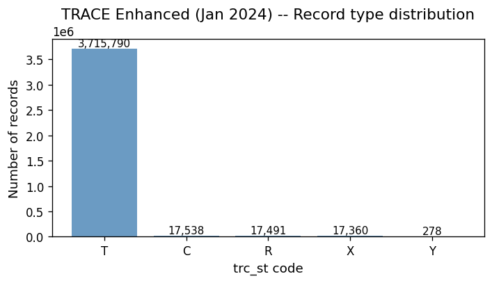
../_images/3d938e17e6e4f0cbd93b80b0f238e3e67d6821ab462d65d07766b8e9e7419c64.png

The large number of C (correction) and X (cancellation) records is exactly why the Dick-Nielsen cleaning procedure exists. These are not separate trades—they are amendments to prior trade reports.

Raw price distribution#

Raw data contains extreme prices from decimal-shift errors, data entry mistakes, and pre-cancellation records. The log-scale histogram reveals a long tail, while the right panel shows the “true” distribution concentrated near par (~100).

raw_prices = raw.select("rptd_pr").collect()["rptd_pr"].to_numpy()

fig, axes = plt.subplots(1, 2, figsize=(12, 4))

axes[0].hist(
    raw_prices[np.isfinite(raw_prices)],
    bins=200,
    color="steelblue",
    alpha=0.7,
    edgecolor="none",
)
axes[0].set_xlabel("Reported price ($)")
axes[0].set_ylabel("Frequency")
axes[0].set_title("Raw prices -- full range (log scale)")
axes[0].set_yscale("log")

mask = (raw_prices > 0) & (raw_prices <= 250)
axes[1].hist(raw_prices[mask], bins=200, color="darkorange", alpha=0.7, edgecolor="none")
axes[1].set_xlabel("Reported price ($)")
axes[1].set_ylabel("Frequency")
axes[1].set_title("Raw prices -- 0 < price <= $250")

fig.tight_layout()
plt.show()

print(f"Prices <= 0:   {(raw_prices <= 0).sum():,}")
print(f"Prices > 1000: {(raw_prices[np.isfinite(raw_prices)] > 1000).sum():,}")
print(f"Null prices:   {np.isnan(raw_prices).sum():,}")

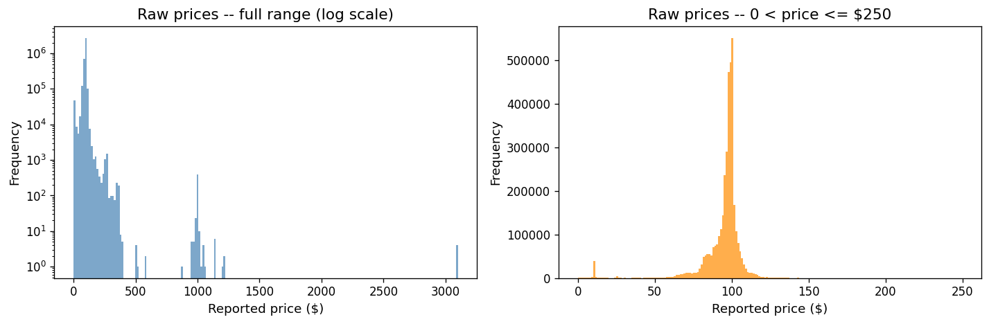
../_images/d2be7e7041b2dcbede696a685c8b4c64cb80990e204108213af3ca06abd02745.png

Prices <= 0:   0
Prices > 1000: 29
Null prices:   0

A single bond’s intraday trades#

To build intuition, let’s look at a single well-traded bond across one day. We plot every TRACE record colored by its status code.

top_cusips = (
    raw.filter(pl.col("trc_st") == "T")
    .group_by("cusip_id")
    .agg(pl.len().alias("n"))
    .sort("n", descending=True)
    .head(5)
    .collect()
)
print("Top 5 CUSIPs by original-trade count (Jan 2024):")
top_cusips

Top 5 CUSIPs by original-trade count (Jan 2024):

shape: (5, 2)

cusip_id	n
str	u32
"95000U3B7"	16722
"126650CX6"	5750
"06051GFM6"	5477
"718172CW7"	4992
"20030NCT6"	4384

# Find a cusip-date pair that has multiple status codes (T, C, X, etc.)
# so the scatter plot illustrates the lifecycle records.
_cusip_date_mix = (
    raw.group_by("cusip_id", "trd_exctn_dt")
    .agg(
        pl.col("trc_st").n_unique().alias("n_status"),
        pl.len().alias("n_records"),
    )
    .filter(pl.col("n_status") >= 3)
    .sort("n_records", descending=True)
    .head(1)
    .collect()
)

# Fall back to the most-traded cusip on 2024-01-16 if no multi-status pair found
if len(_cusip_date_mix) > 0:
    example_cusip = _cusip_date_mix["cusip_id"][0]
    example_date = _cusip_date_mix["trd_exctn_dt"][0]
else:
    example_cusip = top_cusips["cusip_id"][0]
    example_date = None

intraday = (
    raw.filter(
        (pl.col("cusip_id") == example_cusip)
        & (
            (pl.col("trd_exctn_dt") == example_date)
            if example_date is not None
            else (pl.col("trd_exctn_dt") == pl.lit("2024-01-16").str.to_date())
        )
    )
    .sort("trd_exctn_tm")
    .collect()
)

# If the chosen date is empty, fall back to the first available date
if len(intraday) == 0:
    first_date = (
        raw.filter(pl.col("cusip_id") == example_cusip)
        .select(pl.col("trd_exctn_dt").min())
        .collect()
        .item()
    )
    intraday = (
        raw.filter(
            (pl.col("cusip_id") == example_cusip)
            & (pl.col("trd_exctn_dt") == first_date)
        )
        .sort("trd_exctn_tm")
        .collect()
    )

# Convert trd_exctn_tm to hours for plotting
tm_col = intraday["trd_exctn_tm"]
if tm_col.dtype in (pl.Int64, pl.UInt64, pl.Float64):
    times_hrs = tm_col.to_numpy().astype("float64") / 1e9 / 3600
elif tm_col.dtype == pl.Duration:
    times_hrs = tm_col.dt.total_seconds().to_numpy().astype("float64") / 3600
elif tm_col.dtype == pl.Time:
    times_hrs = (
        tm_col.dt.hour().cast(pl.Float64)
        + tm_col.dt.minute().cast(pl.Float64) / 60
        + tm_col.dt.second().cast(pl.Float64) / 3600
    ).to_numpy()
else:
    # String HH:MM:SS
    parts = tm_col.str.split(":")
    times_hrs = (
        parts.list.get(0).cast(pl.Float64)
        + parts.list.get(1).cast(pl.Float64) / 60
        + parts.list.get(2).cast(pl.Float64) / 3600
    ).to_numpy()

trade_date = intraday["trd_exctn_dt"][0]
prices = intraday["rptd_pr"].to_numpy()
statuses = intraday["trc_st"].to_list()

colors_map = {"T": "steelblue", "X": "red", "C": "orange", "W": "purple", "Y": "green"}

fig, ax = plt.subplots(figsize=(10, 4))
for status in sorted(set(statuses)):
    mask_s = np.array([s == status for s in statuses])
    size = 200 if status in ("C", "R") else 25
    ax.scatter(
        times_hrs[mask_s],
        prices[mask_s],
        label=f"trc_st={status}",
        alpha=0.7,
        s=size,
        color=colors_map.get(status, "gray"),
    )
ax.set_xlabel("Hour of day")
ax.set_ylabel("Reported price ($)")
ax.set_title(f"Intraday trades for {example_cusip} on {trade_date}")
ax.legend(fontsize=9)
fig.tight_layout()
plt.show()

print(f"Total records: {len(intraday)}")
for st in sorted(set(statuses)):
    print(f"  trc_st={st}: {statuses.count(st)}")

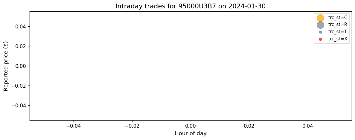
../_images/d990d26bbb1116822f6872dda42a78f3cacc8b7a87eeba73eb2f7dcad7c34879.png

Total records: 10192
  trc_st=C: 1
  trc_st=R: 1
  trc_st=T: 5126
  trc_st=X: 5064

Cancellations (red) and corrections (orange) are not independent trades. They reference prior records via orig_msg_seq_nb and must be matched and removed or replaced. This is the job of the Dick-Nielsen procedure.

4. FISD Universe Filtering#

Before cleaning trade data, we restrict to standard US corporate bonds using the Mergent Fixed Income Securities Database (FISD). The universe is built with these screens:

USD denominated only
Fixed-rate coupon (exclude variable)
Non-convertible
Non-asset-backed
Exclude government, municipal, MBS, ABS, and other non-corporate types
Valid coupon frequency
Complete accrual fields (offering_date, dated_date)
Principal amount = $1,000
Exclude equity-linked / index-linked bonds
Tenor >= 1 year

We then inner-join TRACE on cusip_id with the FISD universe, dropping all non-matching bonds.

fisd = pl.scan_parquet(DATA_DIR / "fisd_universe.parquet")
n_fisd = fisd.select(pl.len()).collect().item()
print(f"FISD Universe: {n_fisd:,} bonds")

FISD Universe: 111,727 bonds

Example bonds from the FISD universe#

fisd.head(5).collect()

shape: (5, 22)

complete_cusip	issue_id	issue_name	issuer_id	foreign_currency	coupon_type	coupon	convertible	asset_backed	rule_144a	bond_type	private_placement	interest_frequency	dated_date	day_count_basis	offering_date	maturity	principal_amt	offering_amt	country_domicile	sic_code	tenor
str	f64	str	f64	str	str	f64	str	str	str	str	str	i64	date	str	date	date	f64	f64	str	str	f64
"000361AA3"	1.0	"NT"	3.0	"N"	"F"	9.5	"N"	"N"	"N"	"CDEB"	"N"	2	1989-11-01	"30/360"	1989-10-24	2001-11-01	1000.0	65000.0	"USA"	"3720"	12.021903
"000361AB1"	2.0	"NT"	3.0	"N"	"F"	7.25	"N"	"N"	"N"	"CDEB"	"N"	2	1993-10-15	"30/360"	1993-10-12	2003-10-15	1000.0	50000.0	"USA"	"3720"	10.006845
"00077DAB5"	3.0	"MTN"	40263.0	"N"	"F"	4.15	"N"	"N"	"N"	"CMTN"	"N"	2	1994-01-14	"30/360"	1994-01-07	1996-01-12	1000.0	100000.0	"USA"	"6029"	2.01232
"00077DAF6"	4.0	"SUB DEP NT SER B"	40263.0	"N"	"F"	8.25	"N"	"N"	"N"	"USBN"	"N"	2	1994-08-02	"30/360"	1994-07-27	2009-08-01	1000.0	200000.0	"USA"	"6029"	15.014374
"00077TAA2"	5.0	"SUB DEP NT SER B"	40263.0	"N"	"F"	7.75	"N"	"N"	"N"	"CDEB"	"N"	2	1993-05-15	"30/360"	1993-05-20	2023-05-15	1000.0	250000.0	"USA"	"6029"	29.984942

Raw vs FISD-filtered comparison#

fisd_filtered = pl.scan_parquet(
    DATA_DIR / "trace_enhanced_fisd" / "**/*.parquet",
    hive_partitioning=True,
).filter(pl.col("year") == 2024, pl.col("month") == 1)

n_fisd_filtered = fisd_filtered.select(pl.len()).collect().item()

n_cusips_raw = raw.select(pl.col("cusip_id").n_unique()).collect().item()
n_cusips_fisd = fisd_filtered.select(pl.col("cusip_id").n_unique()).collect().item()

print(f"{'':30s} {'Rows':>12s} {'Unique CUSIPs':>15s}")
print(f"{'Raw TRACE Enhanced (Jan 24)':30s} {n_raw:>12,} {n_cusips_raw:>15,}")
print(f"{'After FISD filter':30s} {n_fisd_filtered:>12,} {n_cusips_fisd:>15,}")
print(f"{'Dropped':30s} {n_raw - n_fisd_filtered:>12,} {n_cusips_raw - n_cusips_fisd:>15,}")
pct = 100 * (n_raw - n_fisd_filtered) / n_raw
print(f"\nFISD filter removes {pct:.1f}% of raw trade records.")

                                       Rows   Unique CUSIPs
Raw TRACE Enhanced (Jan 24)       3,768,457          29,998
After FISD filter                 2,792,786          11,940
Dropped                             975,671          18,058

FISD filter removes 25.9% of raw trade records.

The FISD filter removes trades in non-standard bonds (government, MBS, ABS, municipals, convertibles, etc.) that are not the focus of corporate bond research.

5. Stage 0: Dick-Nielsen Cleaning Pipeline#

Stage 0 applies 11 sequential filters to the FISD-filtered intraday data and ends with daily aggregation. The implementation lives in src/stage0/clean_trace_local.py (function _apply_filter_chain).

#	Filter	Purpose
1	Dick-Nielsen	Match and remove cancellations, corrections, reversals; remove agency inter-dealer duplicates
2	Decimal-shift corrector	Fix prices that are 10x, 100x, 0.1x, or 0.01x off from neighboring trades
3	Trading time	Restrict to market hours (disabled by default)
4	Trading calendar	Remove trades on non-trading days (weekends, holidays per NYSE calendar)
5	Price filter	Remove trades with price <= 0 or > $1,000
6	Volume filter	Remove trades with dollar volume < $10,000
7	Bounce-back filter	Detect erroneous price spikes that revert within a few trades
8	Yield-price consistency	Remove rows where the yield field equals the price field (data entry error)
9	Amount outstanding	Remove trades with volume > 50% of offering amount
10	Execution vs maturity	Remove trades executed after the bond’s maturity date
11	Initial price error	Flag extreme price jumps in the first few trades per CUSIP

After all filters, intraday trades are aggregated to one row per (cusip_id, date) with equal-weighted price (prc_ew), volume-weighted price (prc_vw), first/last prices, trade count, and total volume.

Stage 0 output: the daily panel#

s0 = pl.scan_parquet(
    DATA_DIR / "stage0" / "enhanced" / "year=*/month=*/data.parquet",
    hive_partitioning=True,
)

s0_jan = s0.filter(pl.col("year") == 2024, pl.col("month") == 1)
n_s0 = s0_jan.select(pl.len()).collect().item()
s0_cols = s0.collect_schema().names()
print(f"Stage 0 Enhanced (Jan 2024) -- Rows: {n_s0:,} (one row per cusip-day)")
print(f"Columns ({len(s0_cols)}): {s0_cols}")

Stage 0 Enhanced (Jan 2024) -- Rows: 149,135 (one row per cusip-day)
Columns (23): ['cusip_id', 'trd_exctn_dt', 'prc_ew', 'prc_vw', 'prc_vw_par', 'prc_first', 'prc_last', 'prc_hi', 'prc_lo', 'trade_count', 'time_ew', 'time_last', 'qvolume', 'dvolume', 'prc_bid', 'bid_last', 'bid_time_ew', 'bid_time_last', 'prc_ask', 'bid_count', 'ask_count', 'year', 'month']

Example rows#

s0_jan.head(10).collect()

shape: (10, 23)

cusip_id	trd_exctn_dt	prc_ew	prc_vw	prc_vw_par	prc_first	prc_last	prc_hi	prc_lo	trade_count	time_ew	time_last	qvolume	dvolume	prc_bid	bid_last	bid_time_ew	bid_time_last	prc_ask	bid_count	ask_count	year	month
str	datetime[ms]	f64	f64	f64	f64	f64	f64	f64	i64	f64	i32	f64	f64	f64	f64	f64	i32	f64	f64	f64	i64	i64
"00037BAC6"	2024-01-16 00:00:00	89.9055	89.90575	89.90575	89.905	89.906	89.906	89.905	4	57610.0	57610	0.16	0.1438492	null	null	null	null	89.90575	null	2.0	2024	1
"00037BAC6"	2024-01-24 00:00:00	89.658	89.658	89.658	89.658	89.658	89.658	89.658	1	43883.0	43883	1.0	0.89658	null	null	null	null	89.658	null	1.0	2024	1
"00037BAC6"	2024-01-30 00:00:00	90.477	90.477	90.477	90.477	90.477	90.477	90.477	1	57628.0	57628	0.669	0.605291	90.477	90.477	57628.0	57628	null	1.0	0.0	2024	1
"00037BAC6"	2024-01-31 00:00:00	91.183667	91.084617	91.084437	91.276	90.999	91.276	90.999	3	41617.333333	44742	4.338	3.951243	null	null	null	null	90.999	null	1.0	2024	1
"00037BAF9"	2024-01-02 00:00:00	98.217	98.217	98.217	98.217	98.217	98.217	98.217	1	41319.0	41319	0.26	0.2553642	null	null	null	null	98.217	null	1.0	2024	1
"00037BAF9"	2024-01-03 00:00:00	98.611	98.611	98.611	98.611	98.611	98.611	98.611	2	57612.0	57612	2.0	1.97222	null	null	null	null	98.611	null	1.0	2024	1
"00037BAF9"	2024-01-24 00:00:00	97.731	97.731	97.731	97.731	97.731	97.731	97.731	1	51328.0	51328	0.075	0.073298	null	null	null	null	97.731	null	1.0	2024	1
"00037BAF9"	2024-01-29 00:00:00	98.303	98.303	98.303	98.303	98.303	98.303	98.303	1	57635.0	57635	0.1	0.098303	98.303	98.303	57635.0	57635	null	1.0	0.0	2024	1
"00037BAF9"	2024-01-30 00:00:00	98.14664	98.146641	98.14664	98.13883	98.15445	98.15445	98.13883	2	48722.0	48722	0.18	0.176664	null	null	null	null	null	null	null	2024	1
"00037BAF9"	2024-01-31 00:00:00	98.489	98.394401	98.394373	98.597	98.381	98.597	98.381	2	60076.5	62503	0.533	0.524442	98.394401	98.381	60076.5	62503	null	2.0	0.0	2024	1

Data reduction through the pipeline#

The table below shows how row counts change at each stage.

raw_both = pl.scan_parquet(
    PULL_DIR / "trace_enhanced" / "**/*.parquet",
    hive_partitioning=True,
    missing_columns="insert",
).select(pl.len()).collect().item()

fisd_both = pl.scan_parquet(
    DATA_DIR / "trace_enhanced_fisd" / "**/*.parquet",
    hive_partitioning=True,
).select(pl.len()).collect().item()

s0_both = s0.select(pl.len()).collect().item()

summary = pl.DataFrame({
    "Stage": [
        "Raw TRACE Enhanced",
        "After FISD filter",
        "Stage 0 (daily panel)",
    ],
    "Rows": [raw_both, fisd_both, s0_both],
    "Granularity": [
        "intraday trade reports",
        "intraday trade reports",
        "one row per cusip-day",
    ],
})
summary

shape: (3, 3)

Stage	Rows	Granularity
str	i64	str
"Raw TRACE Enhanced"	423792457	"intraday trade reports"
"After FISD filter"	329061163	"intraday trade reports"
"Stage 0 (daily panel)"	286454	"one row per cusip-day"

The dramatic reduction from millions of intraday records to the daily panel reflects both (a) removal of erroneous/duplicate records and (b) daily aggregation.

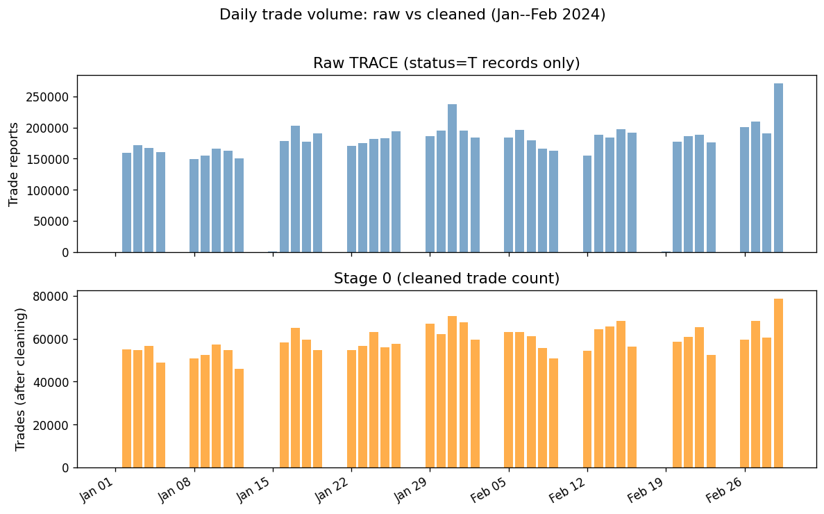
Daily trade counts: raw vs cleaned#

raw_daily = (
    pl.scan_parquet(
        PULL_DIR / "trace_enhanced" / "**/*.parquet",
        hive_partitioning=True,
        missing_columns="insert",
    )
    .filter(
        pl.col("trc_st") == "T",
        pl.col("year") == 2024,
        pl.col("month").is_in([1, 2]),
    )
    .group_by("trd_exctn_dt")
    .agg(pl.len().alias("n_trades"))
    .sort("trd_exctn_dt")
    .collect()
)

s0_daily = (
    s0.filter(pl.col("year") == 2024, pl.col("month").is_in([1, 2]))
    .group_by("trd_exctn_dt")
    .agg(pl.col("trade_count").sum().alias("n_trades"))
    .sort("trd_exctn_dt")
    .collect()
)

fig, axes = plt.subplots(2, 1, figsize=(10, 6), sharex=True)

raw_dates = raw_daily["trd_exctn_dt"].to_pandas()
s0_dates = s0_daily["trd_exctn_dt"].to_pandas()

axes[0].bar(
    raw_dates,
    raw_daily["n_trades"].to_list(),
    color="steelblue",
    alpha=0.7,
    width=0.8,
)
axes[0].set_ylabel("Trade reports")
axes[0].set_title("Raw TRACE (status=T records only)")

axes[1].bar(
    s0_dates,
    s0_daily["n_trades"].to_list(),
    color="darkorange",
    alpha=0.7,
    width=0.8,
)
axes[1].set_ylabel("Trades (after cleaning)")
axes[1].set_title("Stage 0 (cleaned trade count)")
for _ax in axes:
    _ax.xaxis.set_major_locator(mdates.WeekdayLocator(byweekday=mdates.MO))
    _ax.xaxis.set_major_formatter(mdates.DateFormatter("%b %d"))
plt.setp(axes[1].get_xticklabels(), rotation=30, ha="right")

fig.suptitle(
    "Daily trade volume: raw vs cleaned (Jan--Feb 2024)", fontsize=13, y=1.02
)
fig.tight_layout()
plt.show()

../_images/99eb0fe7a23ec26bb1260e4177b1446bc1d30dd0ae34ecf4a295f00c5816a89d.png

Price distributions: raw vs cleaned#

raw_pr = (
    pl.scan_parquet(
        PULL_DIR / "trace_enhanced" / "**/*.parquet",
        hive_partitioning=True,
        missing_columns="insert",
    )
    .filter(
        (pl.col("trc_st") == "T")
        & (pl.col("year") == 2024)
        & (pl.col("month") == 1)
    )
    .select("rptd_pr")
    .collect()["rptd_pr"]
    .to_numpy()
)

s0_pr = (
    s0_jan.select("prc_ew").collect()["prc_ew"].to_numpy()
)

fig, ax = plt.subplots(figsize=(10, 4))
bins = np.linspace(0, 200, 200)
ax.hist(
    raw_pr[(raw_pr > 0) & (raw_pr <= 200)],
    bins=bins,
    alpha=0.5,
    label="Raw (T records)",
    color="steelblue",
    density=True,
)
ax.hist(
    s0_pr[(s0_pr > 0) & (s0_pr <= 200)],
    bins=bins,
    alpha=0.5,
    label="Stage 0 (prc_ew)",
    color="darkorange",
    density=True,
)
ax.set_xlabel("Price ($)")
ax.set_ylabel("Density")
ax.set_title("Price distribution: raw intraday trades vs Stage 0 daily EW price (Jan 2024)")
ax.legend()
fig.tight_layout()
plt.show()

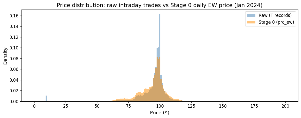
../_images/0c484dec961fbaeb952d93f9f7373afe863a25b2b4ce55177a37b4dfe470c1a8.png

The cleaned distribution is tighter, with extreme tails removed. Daily aggregation (averaging across trades) further reduces noise.

Equal-weighted vs volume-weighted prices#

The Stage 0 panel provides both prc_ew (equal-weighted average across all intraday trades) and prc_vw (volume-weighted). For research, volume-weighted prices down-weight small “noise” trades, providing a better estimate of the bond’s true price.

s0_prices = (
    s0_jan.select("prc_ew", "prc_vw").collect()
)

fig, ax = plt.subplots(figsize=(6, 6))
ax.scatter(
    s0_prices["prc_ew"].to_numpy(),
    s0_prices["prc_vw"].to_numpy(),
    alpha=0.1,
    s=3,
    color="steelblue",
)
lims = [0, 200]
ax.plot(lims, lims, "k--", linewidth=0.8, alpha=0.5)
ax.set_xlabel("EW price ($)")
ax.set_ylabel("VW price ($)")
ax.set_title("Equal-weighted vs volume-weighted daily prices (Jan 2024)")
ax.set_xlim(lims)
ax.set_ylim(lims)
fig.tight_layout()
plt.show()

diff = np.abs(s0_prices["prc_ew"].to_numpy() - s0_prices["prc_vw"].to_numpy())
print(f"Mean |EW - VW| difference:   ${np.nanmean(diff):.4f}")
print(f"Median |EW - VW| difference: ${np.nanmedian(diff):.4f}")
print(f"95th pctile |EW - VW|:       ${np.nanpercentile(diff, 95):.4f}")

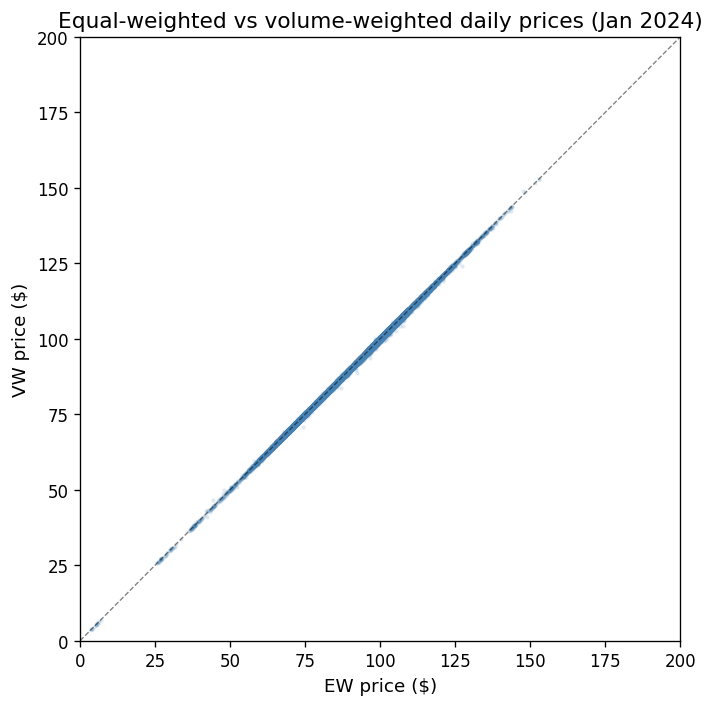
../_images/39255dc97e4bc74c176fd5963b9098135e29c01c15887de9bbff14d6842ccb7b.png

Mean |EW - VW| difference:   $0.0629
Median |EW - VW| difference: $0.0220
95th pctile |EW - VW|:       $0.2612

Market microstructure noise in context#

Most points lie on the 45-degree line, but the divergences—where small trades transact at systematically different prices than large trades—are precisely the market microstructure noise (MMN) that Dickerson, Robotti, and Rossetti (2024) warn about.

Key implications from DRR (2024):

Even after cleaning, daily prices contain MMN because individual trades include bid-ask bounce and dealer markups.
The EW price gives equal weight to a $10K retail trade and a $5M institutional block—yet these trades occur at systematically different prices.
The VW price partially mitigates this, but does not fully remove MMN.
Using noisy prices as signals for portfolio sorts creates spurious predictability. For example, short-term reversal premia of 0.90%/month vanish after MMN correction.
Volume-weighted prices (prc_vw) should be preferred over prc_ew when computing returns for research.

6. Stage 1: Enrichment#

Stage 1 takes the clean daily panel from Stage 0 and enriches it with bond analytics and reference data:

Analytics (computed via QuantLib):

Accrued interest (to convert between clean and dirty prices)
Yield to maturity (YTM)
Modified duration and Macaulay duration
Convexity
Credit spread (bond yield minus duration-matched Liu-Wu Treasury zero-coupon yield)

Merged reference data:

FISD bond characteristics (coupon, maturity, offering amount, callable flag)
Credit ratings from Moody’s and S&P (as-of, forward-filled)
Fama-French 17/30 industry classification (via SIC codes)
Equity identifiers (PERMNO, PERMCO, GVKEY) via the OBAP bond-firm linker

import glob

s1_files = sorted(glob.glob(str(DATA_DIR / "stage1" / "stage1_*.parquet")))
s1_path = s1_files[-1]  # most recent
s1 = pl.scan_parquet(s1_path)
n_s1 = s1.select(pl.len()).collect().item()
cols_s1 = s1.collect_schema().names()
print(f"Stage 1 ({Path(s1_path).name}) -- Rows: {n_s1:,}  |  Columns: {len(cols_s1)}")
print(f"Columns: {cols_s1}")

Stage 1 (stage1_20260223.parquet) -- Rows: 333,901  |  Columns: 43
Columns: ['cusip_id', 'permno', 'permco', 'gvkey', 'trd_exctn_dt', 'pr', 'prfull', 'acclast', 'accpmt', 'accall', 'ytm', 'mod_dur', 'mac_dur', 'convexity', 'bond_maturity', 'credit_spread', 'prc_ew', 'prc_vw_par', 'prc_first', 'prc_last', 'prc_hi', 'prc_lo', 'trade_count', 'time_ew', 'time_last', 'qvolume', 'dvolume', 'prc_bid', 'bid_last', 'bid_time_ew', 'bid_time_last', 'prc_ask', 'bid_count', 'ask_count', 'db_type', 'ff17num', 'ff30num', 'bond_age', 'bond_amt_outstanding', 'sp_rating', 'mdy_rating', 'spc_rating', 'mdc_rating']

Example rows#

s1.head(10).collect()

shape: (10, 43)

cusip_id	permno	permco	gvkey	trd_exctn_dt	pr	prfull	acclast	accpmt	accall	ytm	mod_dur	mac_dur	convexity	bond_maturity	credit_spread	prc_ew	prc_vw_par	prc_first	prc_last	prc_hi	prc_lo	trade_count	time_ew	time_last	qvolume	dvolume	prc_bid	bid_last	bid_time_ew	bid_time_last	prc_ask	bid_count	ask_count	db_type	ff17num	ff30num	bond_age	bond_amt_outstanding	sp_rating	mdy_rating	spc_rating	mdc_rating
cat	i32	i32	i32	datetime[ns]	f32	f32	f32	f32	f32	f64	f32	f32	f32	f32	f64	f32	f32	f32	f32	f32	f32	i16	f32	i32	f32	f32	f32	f32	f32	f32	f32	i16	i16	i8	i8	i8	f32	i64	i8	i8	i8	i8
"00033GAA3"	null	null	null	2024-01-12 00:00:00	99.644699	99.64473	0.0	0.0	0.0	0.084359	4.018	4.187	19.893	5.01	0.046275	99.662743	99.64463	99.75	99.5	100.080002	99.5	47	32683.873047	55470	43.099998	42.946835	99.606499	99.5	33551.53125	55470.0	99.813789	17	5	3	16	29	0.002738	525000	14	15	14	15
"00033GAA3"	null	null	null	2024-01-16 00:00:00	98.920601	98.920624	0.0	0.0	0.0	0.086234	4.008	4.181	19.813	4.999	0.047138	98.936501	98.919998	99.5	98.949997	99.5	98.625	20	45762.851562	55865	17.25	17.0637	98.970909	98.6875	39102.855469	52321.0	99.028244	7	6	3	16	29	0.013689	525000	14	15	14	15
"00033GAA3"	null	null	null	2024-01-17 00:00:00	96.936501	96.936493	0.0	0.0	0.0	0.091364	3.986	4.168	19.632999	4.997	0.051367	96.930786	96.930786	98.030998	96.0	98.030998	96.0	14	51371.070312	63216	14.0	13.57031	97.00193	96.75	49492.5	53847.0	96.787689	4	9	3	16	29	0.016427	525000	14	15	14	15
"00033GAA3"	null	null	null	2024-01-18 00:00:00	97.560303	97.56031	0.0	0.0	0.0	0.089939	3.983	4.163	19.608999	4.994	0.049759	97.559998	97.559998	97.625	97.25	97.75	97.25	5	46109.199219	54864	5.0	4.878	97.45858	97.25	46403.332031	54864.0	97.712517	3	2	3	16	29	0.019165	525000	14	15	14	15
"00033GAA3"	null	null	null	2024-01-19 00:00:00	97.666901	97.690155	0.023264	0.0	0.023264	0.089667	3.982	4.16	19.594999	4.991	0.04948	97.800003	97.666664	97.599998	98.0	98.0	97.599998	2	53709.0	54910	1.2	1.172	null	null	null	null	97.666893	null	2	3	16	29	0.021903	525000	14	15	14	15
"00033GAA3"	null	null	null	2024-01-22 00:00:00	97.141998	97.188507	0.046528	0.0	0.046528	0.091023	3.974	4.155	19.531	4.983	0.051037	97.141846	97.141846	97.195	97.5	97.5	97.0	19	53547.632812	59996	19.0	18.456949	97.123344	97.375	53735.855469	59911.0	97.267708	7	4	3	16	29	0.030116	525000	14	15	14	15
"00033GAA3"	null	null	null	2024-01-23 00:00:00	96.408501	96.478279	0.069792	0.0	0.069792	0.092933	3.964	4.148	19.450001	4.98	0.052799	96.372002	96.408134	96.75	96.25	96.75	96.223999	7	53864.144531	60691	5.5	5.302447	96.402405	96.25	54821.75	60691.0	96.375	4	1	3	16	29	0.032854	525000	14	15	14	15
"00033GAA3"	null	null	null	2024-01-24 00:00:00	95.909401	96.002426	0.093056	0.0	0.093056	0.094246	3.957	4.143	19.388	4.977	0.05366	95.783333	95.907265	96.808998	94.882004	96.808998	94.859001	6	44907.5	55726	3.6	3.452662	95.673523	94.859001	49877.0	55726.0	96.169693	2	3	3	16	29	0.035592	525000	14	15	14	15
"00033GAA3"	null	null	null	2024-01-25 00:00:00	95.077301	95.240166	0.162847	0.0	0.162847	0.096461	3.94	4.131	19.254999	4.975	0.056679	95.077003	95.077003	95.25	94.903999	95.25	94.903999	2	40048.5	47720	2.0	1.90154	95.25	95.25	32377.0	32377.0	null	1	0	3	16	29	0.03833	525000	14	15	14	15
"00033GAA3"	null	null	null	2024-01-26 00:00:00	95.041801	95.227921	0.186111	0.0	0.186111	0.096561	3.937	4.128	19.229	4.972	0.05642	95.041664	95.041664	95.125	95.125	95.125	94.875	3	48799.332031	54143	3.0	2.85125	94.875	94.875	47008.0	47008.0	95.125	1	2	3	16	29	0.041068	525000	14	15	14	15

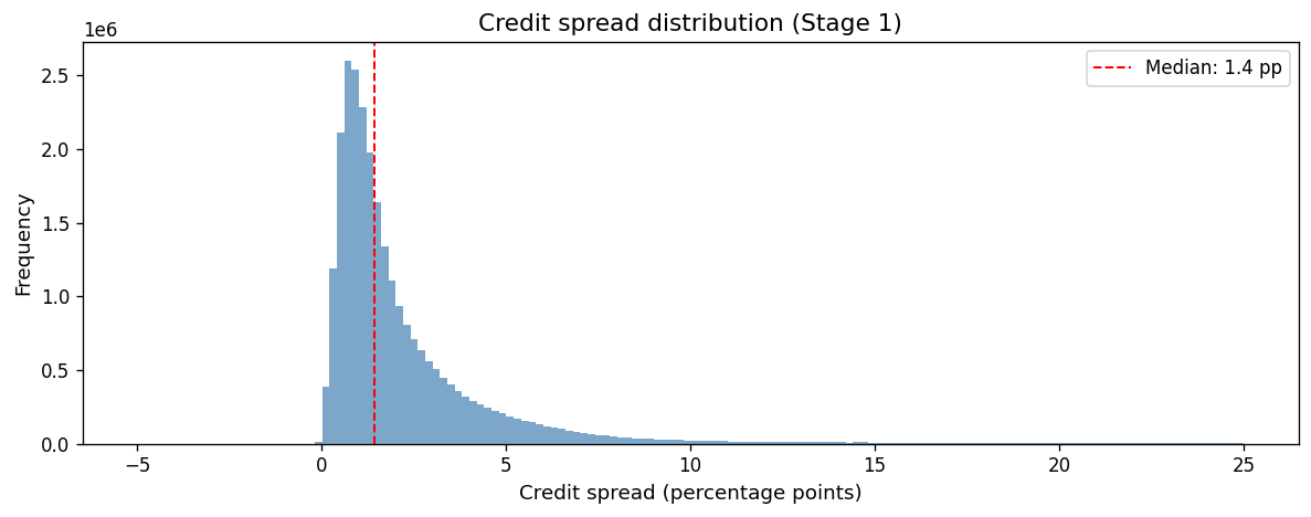
Credit spread distribution#

The credit spread is the yield premium a corporate bond pays over a duration-matched Treasury zero-coupon yield. It reflects credit risk, liquidity risk, and other bond-specific factors.

cs = (
    s1.filter(
        pl.col("credit_spread").is_not_null()
        & (pl.col("credit_spread") > -0.05)
        & (pl.col("credit_spread") < 0.25)
    )
    .select("credit_spread")
    .collect()["credit_spread"]
    .to_numpy()
)

fig, ax = plt.subplots(figsize=(10, 4))
ax.hist(cs * 100, bins=150, color="steelblue", alpha=0.7, edgecolor="none")
median_cs = np.median(cs) * 100
ax.axvline(
    median_cs,
    color="red",
    linestyle="--",
    linewidth=1.2,
    label=f"Median: {median_cs:.1f} pp",
)
ax.set_xlabel("Credit spread (percentage points)")
ax.set_ylabel("Frequency")
ax.set_title("Credit spread distribution (Stage 1)")
ax.legend()
fig.tight_layout()
plt.show()

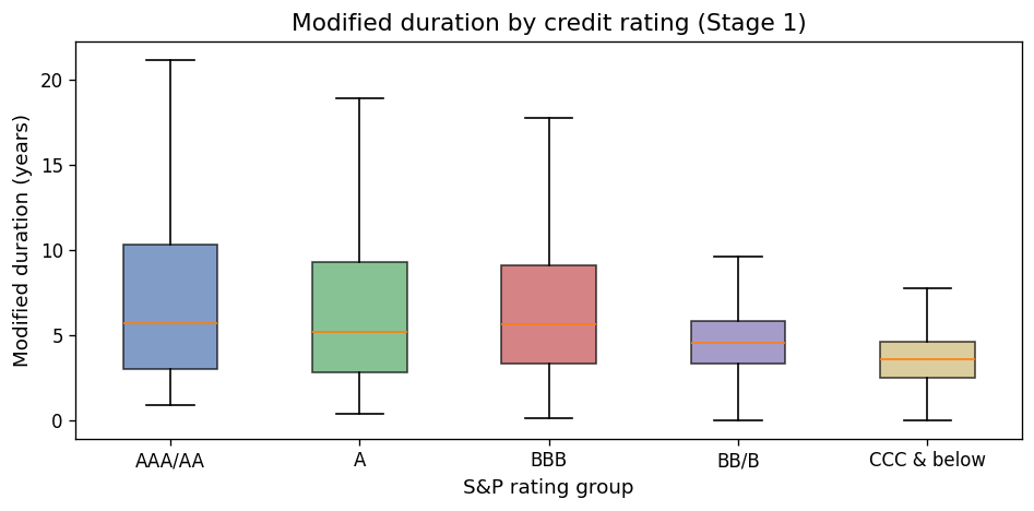
../_images/e463264968d0f6e11c56d8e1c9ac147bb059cc4d8d9575cd1c28d358ea47b81f.png

Modified duration by credit rating#

Investment-grade bonds (AAA through BBB) tend to have longer duration because they carry lower default risk and can issue at longer maturities. High-yield bonds (BB and below) tend to have shorter duration.

s1_dur = (
    s1.filter(
        pl.col("mod_dur").is_not_null()
        & pl.col("sp_rating").is_not_null()
        & (pl.col("mod_dur") > 0)
        & (pl.col("mod_dur") < 30)
        & (pl.col("sp_rating") > 0)
    )
    .select("mod_dur", "sp_rating")
    .collect()
)


def _rating_bucket(r):
    if r <= 3:
        return "AAA/AA"
    elif r <= 6:
        return "A"
    elif r <= 10:
        return "BBB"
    elif r <= 16:
        return "BB/B"
    else:
        return "CCC & below"


s1_dur_pd = s1_dur.to_pandas()
s1_dur_pd["rating_group"] = s1_dur_pd["sp_rating"].apply(_rating_bucket)

order = ["AAA/AA", "A", "BBB", "BB/B", "CCC & below"]
data_by_group = [
    s1_dur_pd.loc[s1_dur_pd["rating_group"] == g, "mod_dur"].values
    for g in order
]
# Only keep groups with data
valid = [(g, d) for g, d in zip(order, data_by_group) if len(d) > 0]
order_valid = [g for g, _ in valid]
data_valid = [d for _, d in valid]

fig, ax = plt.subplots(figsize=(8, 4))
bp = ax.boxplot(data_valid, labels=order_valid, patch_artist=True, showfliers=False)
box_colors = ["#4c72b0", "#55a868", "#c44e52", "#8172b2", "#ccb974"]
for i, patch in enumerate(bp["boxes"]):
    patch.set_facecolor(box_colors[i % len(box_colors)])
    patch.set_alpha(0.7)
ax.set_xlabel("S&P rating group")
ax.set_ylabel("Modified duration (years)")
ax.set_title("Modified duration by credit rating (Stage 1)")
fig.tight_layout()
plt.show()

/var/folders/l3/tj6vb0ld2ys1h939jz0qrfrh0000gn/T/ipykernel_93385/3343011909.py:41: MatplotlibDeprecationWarning: The 'labels' parameter of boxplot() has been renamed 'tick_labels' since Matplotlib 3.9; support for the old name will be dropped in 3.11.
  bp = ax.boxplot(data_valid, labels=order_valid, patch_artist=True, showfliers=False)

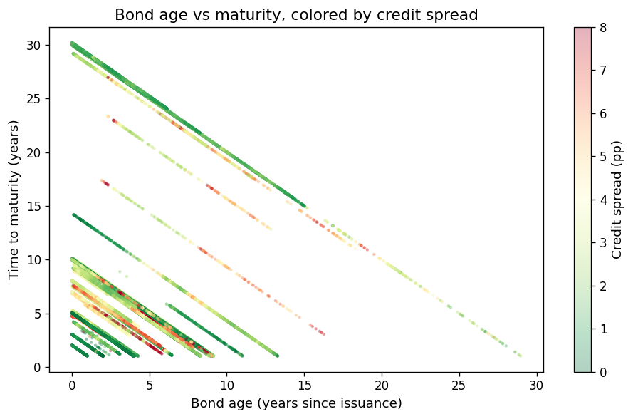
../_images/24516082c9a3530e6b45d162cd82883d53c0544894af12bfeb513fe86a455bdd.png

Bond age vs time-to-maturity#

s1_scatter = (
    s1.filter(
        pl.col("bond_maturity").is_not_null()
        & pl.col("bond_age").is_not_null()
        & pl.col("credit_spread").is_not_null()
        & (pl.col("credit_spread") > -0.02)
        & (pl.col("credit_spread") < 0.20)
        & (pl.col("bond_maturity") > 0)
        & (pl.col("bond_maturity") < 35)
    )
    .select("bond_age", "bond_maturity", "credit_spread")
    .head(50_000)
    .collect()
)

fig, ax = plt.subplots(figsize=(8, 5))
sc = ax.scatter(
    s1_scatter["bond_age"].to_numpy(),
    s1_scatter["bond_maturity"].to_numpy(),
    c=s1_scatter["credit_spread"].to_numpy() * 100,
    s=3,
    alpha=0.3,
    cmap="RdYlGn_r",
    vmin=0,
    vmax=8,
)
cbar = fig.colorbar(sc, ax=ax)
cbar.set_label("Credit spread (pp)")
ax.set_xlabel("Bond age (years since issuance)")
ax.set_ylabel("Time to maturity (years)")
ax.set_title("Bond age vs maturity, colored by credit spread")
fig.tight_layout()
plt.show()

../_images/1725a99532e4f72f4d88585f7b18795c13ab037e5735a59591b078e5bee83e0a.png

7. Takeaways and Best Practices#

Always clean TRACE data before computing returns. Raw data contains cancellations, corrections, reversals, decimal-shift errors, and bounce-back errors. Using uncleaned data biases return estimates.
Use the FISD universe to restrict to standard US corporate bonds. Mixing in government, muni, ABS, or MBS trades will contaminate your sample.
Prefer volume-weighted prices (prc_vw) over equal-weighted (prc_ew) when computing returns. EW prices over-weight small, noisy trades.
Be aware of market microstructure noise. Even after cleaning, daily prices contain bid-ask bounce and dealer markup noise (Dickerson, Robotti, and Rossetti, 2024). Price-based signals (e.g., short-term reversal) may be spuriously profitable.
Avoid ex-post filtering. Do not condition your bond sample on future price availability or forward-looking criteria. Use only ex-ante filters with information available at portfolio formation (Dickerson, Robotti, and Rossetti, 2024, 2026).
Validate against known benchmarks. Compare your output to the Open Bond Asset Pricing (OBAP) database for duration, convexity, and credit spread validation.

References#

Dick-Nielsen, J. (2009). Liquidity biases in TRACE. Journal of Fixed Income, 19(2), 43–55.
Dick-Nielsen, J. (2014). How to clean enhanced TRACE data. Working paper.
Dickerson, A., Robotti, C., and Rossetti, G. (2024). Common pitfalls in the evaluation of corporate bond strategies. Available at SSRN: https://ssrn.com/abstract=4575879.
Dickerson, A., Robotti, C., and Rossetti, G. (2026). The Corporate Bond Factor Replication Crisis.

Cleaning TRACE Corporate Bond Data: A Walkthrough

Contents

Cleaning TRACE Corporate Bond Data: A Walkthrough#

1. What Is TRACE and Why Does Cleaning Matter?#

What securities does TRACE cover?#

What information is in the public data?#

Data access#

Why this pipeline exists: lessons from the literature#

Pipeline overview#

2. Data Sources and Pipeline Overview#

Three TRACE feeds#

FISD reference data (6 files)#

Liu-Wu Treasury yields#

Fama-French SIC codes#

Open Source Bond Asset Pricing (OSBAP) datasets#

3. Raw TRACE Enhanced Data#

Example rows#

TRACE status code distribution#

Raw price distribution#

A single bond’s intraday trades#

4. FISD Universe Filtering#

Example bonds from the FISD universe#

Raw vs FISD-filtered comparison#

5. Stage 0: Dick-Nielsen Cleaning Pipeline#

Stage 0 output: the daily panel#

Example rows#

Data reduction through the pipeline#

Daily trade counts: raw vs cleaned#

Price distributions: raw vs cleaned#

Equal-weighted vs volume-weighted prices#

Market microstructure noise in context#

6. Stage 1: Enrichment#

Example rows#

Credit spread distribution#

Modified duration by credit rating#

Bond age vs time-to-maturity#

7. Takeaways and Best Practices#

References#