Case Study: Hedging Oil Price Exposure As An E&P

Case Study: Hedging Oil Price Exposure As An E&P#

import pandas as pd
import numpy as np


import plotly.io as pio

from IPython.display import display

import warnings


# import hedging functions
import brent_hedging_functions as hf


warnings.filterwarnings("ignore")
pio.templates.default = "plotly_white"
pd.set_option("display.max_columns", None)
COMDTY_CODES = {"brent": "CB"}
# cme month codes dict
cme_month_codes = {
    1: "F",
    2: "G",
    3: "H",
    4: "J",
    5: "K",
    6: "M",
    7: "N",
    8: "Q",
    9: "U",
    10: "V",
    11: "X",
    12: "Z",
}

Introduction to OptiQuant Analytics#

OptiQuant Analytics is a finance and strategy consultancy specializing in the upstream energy sector. We focus on developing financial models and data analytics frameworks to support risk management, capital allocation, and strategic decision-making for companies and investors in the energy space.

Clients & Industry Focus We primarily work with:

Oil & Gas Producers
- Also known as Exploration & Production (E&P) companies or upstream operators.
- These firms extract, process, and sell crude oil, natural gas, and natural gas liquids (NGLs).
Private Equity Firms
- Investors that own, acquire, or manage upstream energy companies.
- Require robust financial models for valuation, risk assessment, and capital allocation.

Core Areas of Expertise We apply quantitative finance, risk modeling, and economic analysis to help upstream energy firms make data-driven financial decisions. Our key areas of focus include:

Corporate Hedging Advisory & Risk Modeling
- Structuring and evaluating commodity hedging strategies
- Assessing hedge effectiveness and risk exposure
Data Modeling, Integration & Analytics
- Automating financial and operational data workflows
- Developing analytical tools for market and company-level insights
Financial Strategy & Capital Allocation
- Evaluating investment opportunities and capital structuring
- Scenario modeling for debt, equity, and cash flow planning
Corporate Valuation & Cash Flow Modeling
- Building financial projections for M&A, fundraising, and strategic planning
- Quantifying the impact of commodity price fluctuations on valuation
Macroeconomic & Market Analysis
- Assessing trends in interest rates, inflation, and economic cycles
- Understanding supply, demand, and pricing dynamics in global energy markets

Background & Experience

15+ Years in finance, energy, and investment strategy:

Energy Investment Banking (5 years): Focused on M&A, capital markets, and financial advisory at Morgan Stanley and Jefferies
Private Credit & Structured Investments (3 years): Generalist private credit investing at Deerpath Capital Management and Crestline Investors
Upstream Energy Finance Leadership (4 years): VP of Finance at Triple Crown Resources, a private equity-backed upstream operator
Financial Analytics & Decision Support (3 years): Developing financial models & strategic tools for energy firms at OptiQuant Analytics

Education

🎓 BA in Mathematical Economic Analysis – Rice University (2010)
🎓 MS in Financial Mathematics – University of Chicago (2024)

Case Study: Hedging Oil Price Exposure As An E&P#

What is an “E&P”?#

Exploration and production businesses in the oil and gas sector are companies that extract oil and gas from the ground, and sell these commodities to the market. Extraction is via the drilling and operation of oil and gas wells. Also called “upstream” companies.
Employ a broad range of skillsets (PhDs/Engineering masters for scientific and geological work, MBAs / finance for management, GEDs or simply years of experience for “on-the-ground” field work).
Capital-intensive businesses, challenging to operate for a variety of reasons, but can be very lucrative for shareholders if growth and financial risk are managed well.
Financial risk $\rightarrow$ probability of loss of investment. For E&Ps, this investment risk arises from large minimum capital investment required to drill and operate an oil or gas well:
1. Seismic and geological studies of an area to assess how much oil and gas exists underground can cost anywhere from $200k - $2 million+, depending on the complexity.
2. Drilling a single oil or gas well can cost $5mm - $25mm onshore US, spent over several months. Offshore oil and gas wells can cost $150 million+ (these are considered capital expenditures).
3. Beyond this, there are operating costs, initial processing costs for the company, as well as pipeline or truck transportation expenses.
4. Due to the asset-heavy nature of these businesses, they can typically raise leverage from banks (and more recently, credit funds). Managing this leverage effectively requires a business skillset.
5. Furthermore, the business sells its products at a price reflective of commodity futures markets (with each of oil, natural gas, etc. comprising a separate market, each with its own dynamics).

Primary Business Objectives#

Grow cash flow via higher production of oil, gas, and NGLs (ethane, propane, butane, natural gasoline).
Minimize the risk around future cash flows by de-risking key business areas (geological, financial).
Increase net asset value (equity value)—typically a byproduct of executing the first two objectives well.

Essentially, the E&P management team is trying to maximize the Risk-Adjusted Return on Capital (RAROC) for their investors.

In other words, they aim to maximize expected future cash inflows while minimizing the risk around those future cash inflows.

Maximizing RAROC is essentially a business equivalent of maximizing the “Sharpe Ratio” of an investment portfolio!

Sharpe Ratio for a Portfolio (Reminder)

A higher Sharpe Ratio indicates better risk-adjusted performance. The Sharpe Ratio is defined as:

\[ \text{Sharpe Ratio}_{\text{portfolio}} = \frac{R_p - R_f}{\sigma_p} \]

where:

$ R_p $ = Expected portfolio return
$ R_f $ = Risk-free rate
$ \sigma_p $ = Standard deviation of portfolio returns

Risk-Adjusted Return on Capital (Business)

A higher RAROC indicates better risk-adjusted business performance.

\[\begin{split} \begin{align} \textcolor{teal}{\text{Risk-Adjusted Return on Capital}_{\text{business}}} &= \frac{\textcolor{blue}{\text{Expected Return}} - \textcolor{red}{\text{Risk-Free Return}}}{\text{Expected Deviation of Returns}} \tag{1} \\ \textcolor{blue}{\text{Expected Return}} &= \frac{\textcolor{green}{\text{Expected Future Revenues}} - \textcolor{orange}{\text{Expected Future Costs}}}{\text{Capital Invested}} \tag{2} \\ \textcolor{green}{\text{Expected Future Revenues}} &= (\textcolor{purple}{\text{Expected Future Commodity Prices}} \times \text{Expected Future Volume of Oil/Gas/NGLs}) + \textcolor{purple}{\text{Net Cash Flow Impact of Hedging}} \tag{3} \end{align} \end{split}\]

Primary Source of Revenue Risk: Commodity Prices#

OptiQuant helps clients reduce uncertainty around Equation (3):

\[\begin{split} \begin{align} \textcolor{green}{\text{Expected Future Revenues}} &= (\textcolor{purple}{\text{Expected Future Commodity Prices}} \times \text{Expected Future Volume of Oil/Gas/NGLs}) + \textcolor{purple}{\text{Net Cash Flow Impact of Hedging}} \tag{3} \\ \end{align} \end{split}\]

Defining The Corporate Hedging Problem: How To Reduce Price Risk (Where Revenue = Price x Volume)#

The challenge is captured in Equation (3) and the futures term structure below (for Brent oil, Henry Hub natural gas, and Propane, a natural gas liquid/NGL)

Brent Price History - Last 11 Days

Henry Hub Price History - Last 11 Days

Propane Price History - Last 11 Days

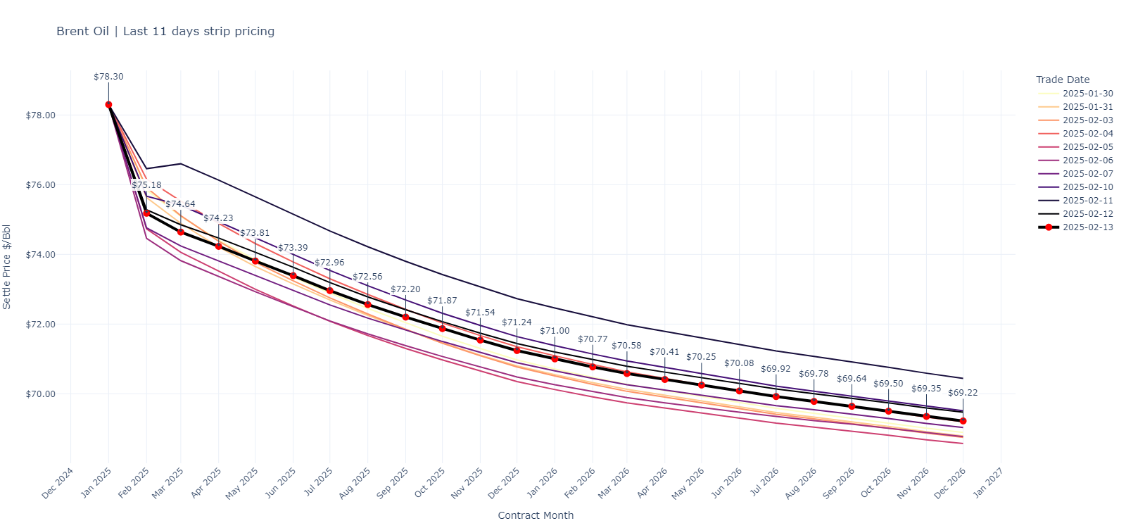
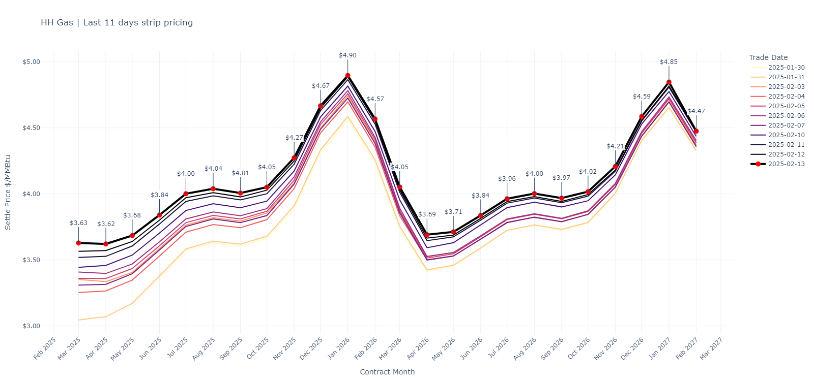
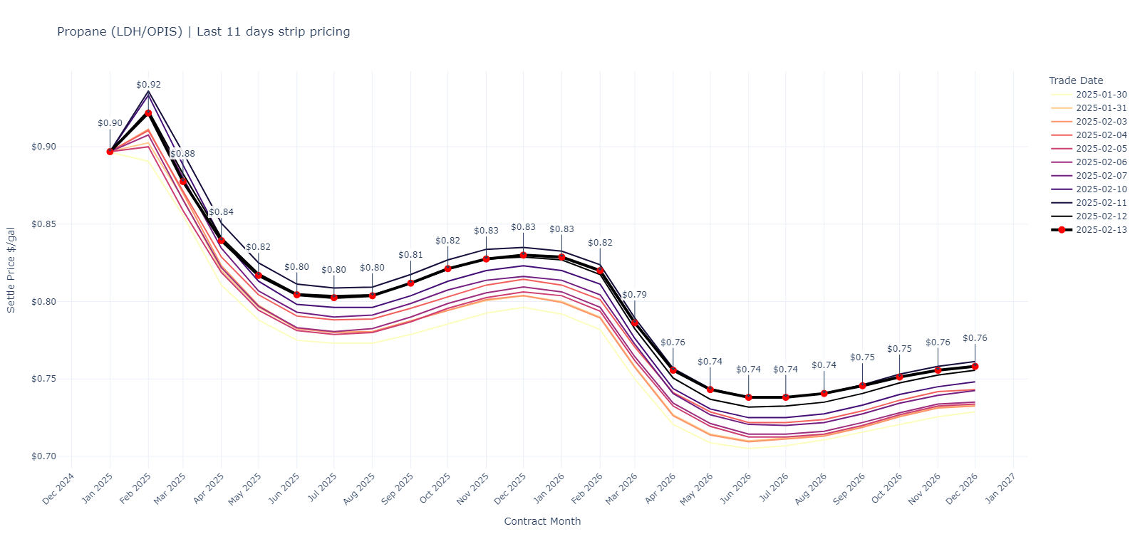
Managing Revenue Risk Via Hedging#

E&Ps have a natural long exposure to oil, natural gas, and NGL prices: Their (unhedged) revenue is therefore stochastic and subject to factors influencing oil and gas prices, including:
- Supply, demand, storage
- Geopolitics
- Interest rates
- Speculative interest
Hedging tools include:
- Calls
- Puts
- Fixed price swaps
- (Rarely) Exotic structures
Many hedging decisions are made without fully considering the underlying statistical properties of the commodities being hedged.

Benefits of Risk Management#

Attract greater capital investment $\rightarrow$ investors prefer companies demonstrating superior financial risk management.
Stronger IPO potential $\rightarrow$ public investors seek companies with predictable multi-year cash flows.
Higher valuation multiples (P/E ratios) $\rightarrow$ companies with higher RAROC command higher premiums in financial markets.
Increased wealth for employees and shareholders

This Lecture:#

☐ 1. Model an E&P as a long position in Brent oil futures (CME: CY).

☐ 2. Work with real option prices & futures data for Brent oil.

☐ 3. Use option delta to approximate the probability of an option expiring in-the-money.

☐ 4. Use option delta to define acceptable risk ranges for the hedging program (e.g., 80% probability of options expiring worthless).

☐ 5. Design a hedging strategy to lock in a price floor for oil using put options.

☐ 6. Attempt to make the hedge costless by selling call options (i.e., constructing a costless collar).

☐ 7. Validate option pricing models using Monte Carlo simulation of Brent futures with implied volatility.

Homework Assignment:#

Replicate this exercise for SPX options.

A Brief Review Of The Option Market and Option Pricing#

! Important !

Model Inputs for Option Pricing#

The underlying security’s current price (Brent, in this case) → Known / observable.
The option strike price → Chosen by the investor; market makers provide quotes for commonly used strikes.
Time to maturity → Chosen by the investor; Brent options are typically quoted in monthly maturities.
The risk-free rate → Observable (commonly estimated using U.S. Treasuries of similar maturity).
The implied volatility → Not observable; it is inferred from market prices by solving the BSM equation.

All inputs to the BSM model are known or observable in the market, except for one: implied volatility (which must be inferred from market prices).

Call Options#

Can buy or sell call options for a price (determined by the market; also called the option “premium” or “cost”).
Option prices vary based on current Brent price level, and future expectations of movement.
Investor chooses strike price, time to expiry (contract maturity), and whether to buy (go long) or sell (short) the call option.
If Brent price at expiry > strike price, a call option is in-the-money (“ITM”), and the buyer receives (Brent – strike) at settlement.
- Net of upfront cost, the call option buyer’s Payoff = (Brent – strike) – upfront cost.
If Brent price at expiry <= strike price, a call option is out-of-the-money (“OTM”), and expires worthless.
- The call option buyer’s Payoff = – upfront cost $\rightarrow$ The buyer loses the amount paid for the option.

Black-Scholes Formula For European Call Option Pricing#

\[ C(S, K, \sigma, r, T) = S \Phi (d_1) - K e^{-rT} \Phi (d_2) \]

where:

$S$ = Price of underlying
$K$ = Option strike price
$\Phi(.)$ = CDF of Standard Normal Distribution
$\sigma$ = Implied volatility (IV) of the underlying asset
$r$ = Risk-free rate
$T$ = Time remaining to expiry
$d_1 = \frac{\ln\left(\frac{S}{K}\right) + \left(r + \frac{\sigma^2}{2}\right)T}{\sigma \sqrt{T}}$
$d_2 = d_1 - \sigma \sqrt{T}$

Call Option Payoff at Expiry#

Parameter	Value
Brent Price	$80.00 per Barrel
Option Strike Price	$90.25 per Barrel
Time to Maturity	0.5 years (6-month option)
Annual Risk-Free Rate	4.3% (6 mo. U.S. Treasury Bill Yield)
Annualized Volatility	27.44% (As of 1/23/25)
Option Price	$3.19 per Barrel

call_payoffs = hf.show_call_option_payoff(S=80, K=90.25, sigma=0.2744, r=0.045, T=0.5)

Put Options#

Same as call options:

Can buy or sell put options for a price (determined by the market; also called the option “premium” or “cost”).
Option prices vary based on current Brent price level, and future expectations of movement.
Investor chooses strike price, time to expiry (contract maturity), and whether to buy (go long) or sell (short) the put option.

Different from call options:

If Brent price at expiry < strike price, a put option is in-the-money (“ITM”), and the buyer receives (strike – Brent) at settlement.
- Net of upfront cost, the put option buyer’s Payoff = (strike – Brent) – upfront cost.
If Brent price at expiry >= strike price, a put option is out-of-the-money (“OTM”), and expires worthless.
- The put option buyer’s Payoff = – upfront cost $\rightarrow$ The buyer loses the amount paid for the option.

Black-Scholes Formula For European Put Option Pricing#

\[ P(S, K, \sigma, r, T) = K e^{-rT} \Phi (-d_2) - S \Phi (-d_1) \]

where:

$S$ = Price of underlying
$K$ = Option strike price
$\Phi(.)$ = CDF of Standard Normal Distribution
$\sigma$ = Implied volatility (IV) of the underlying asset
$r$ = Risk-free rate
$T$ = Time remaining to expiry
$d_1 = \frac{\ln\left(\frac{S}{K}\right) + \left(r + \frac{\sigma^2}{2}\right)T}{\sigma \sqrt{T}}$
$d_2 = d_1 - \sigma \sqrt{T}$

Put Option Payoff at Expiry#

Parameter	Value
Brent Price	$80.00 per Barrel
Option Strike Price	$75.00 per Barrel
Time to Maturity	0.5 years (6-month option)
Annual Risk-Free Rate	4.3% (6 mo. U.S. Treasury Bill Yield)
Annualized Volatility	27.44% (As of 1/23/25)
Option Price	$3.17 per Barrel

put_payoffs = hf.show_put_option_payoff(S=80, K=75, sigma=0.2744, r=0.045, T=0.5)

The Costless Collar: A “Free” Floor on Oil Prices#

collar_payoff = hf.build_costless_collar(
    put_payoffs, call_payoffs, put_strike=75, call_strike=90.25
)
collar_payoff = hf.add_S_payoff(collar_payoff, S0=80, name="Brent")

Observation 1: Locking in the floor is a dynamic decision. Why?

Observation 2: A high floor is a contradictory objective with a high ceiling price. Why?

Question 1: How Do We Know What Strikes / Expiries To Hedge?#

(Partial) Answer: We need some estimate of the probability of the underlying price crossing the call or put strikes (i.e. the prob. of the option expiring in-the-money, $P_{ITM}$).

Question 2: Is There A Metric That Allows Us To Estimate This Probability, Based on Option Prices?#

Quick Answer: Yes - the option delta is a good estimate.

Less Quick Answer: Yes - $\Phi(d_2)$, which is the risk-neutral probability of an option expiring ITM.:

But:

it’s a bit more involved to calculate,
call and put deltas are freely available from many data providers,
$\Phi(d_2)$ is typically fairly close to $\Phi(d_1)$, particularly for options near-the-money or close to expiry ($T\rightarrow 0$),
We can approximate $\Phi(d_2)$ with a first-order Taylor approximation of $\Phi(.)$, since we know the value of the call option delta $\Phi(d_1)$ (and of course, the put option delta $(\Phi(d_1) - 1)$

…and if you really want to know the relationship:

\[\begin{split} \begin{aligned} d_1 &= \frac{ln(S/K) + (r + \frac{\sigma^2}{2})T}{\sigma\sqrt{T}} \\ d_2 &= \frac{ln(S/K) + (r - \frac{\sigma^2}{2})T}{\sigma\sqrt{T}} \\ \\ \Rightarrow d_2 &= d_1 - \sigma\sqrt{T} \rightarrow \textit{Note that } d_2 \le d_1 \\ \\ \\ \text{Since }(d_1 - d_2) &= \sigma\sqrt{T} \text{, we can use a first order Taylor approximation to estimate }\Phi(d_2) \\ \\ \Rightarrow \Phi(d_2) &\approx \Phi(d_1) - \Phi'(d_1) (d_2 - d_1) \\ \\ \Rightarrow \Phi(d_2) &\approx \Phi(d_1) - \frac{e^{-d_1^2/2}}{\sqrt{2\pi}} (\sigma\sqrt{T}) \\ \\ \\ \Rightarrow \Phi(d_2) &\approx \Delta_C - \textit{Adj. Factor} \\ \Rightarrow \Phi(d_2) &\approx \Delta_P - (\textit{Adj. Factor} - 1) \\ \end{aligned} \end{split}\]

\[\begin{split} \begin{aligned} \text{For call options} \rightarrow \Delta_C = \frac{\partial C}{\partial S}&=\Phi(d_1) \\ \text{For put options} \rightarrow \Delta_P = \frac{\partial P}{\partial S}&=\Phi(d_1)-1 \\ \\ \textit{where: } \Phi(d_1) \text{ is the standard normal CDF evaluated at } &d_1 \end{aligned} \end{split}\]

For the rest of this lecture and the homework assignment, we will assume the option delta is an estimate of the probability of that option expiring ITM.

Option Deltas#

Call Option Delta: Measures the sensitivity of the call option’s price to changes in the stock price. It ranges from 0 (deep out-of-the-money) to 1 (deep in-the-money).

\[ \Delta_C = \frac{\partial C}{\partial S} = \Phi (d_1) \]

Put Option Delta: Measures the sensitivity of the put option’s price to changes in the stock price. It ranges from -1 (deep in-the-money) to 0 (deep out-of-the-money).

\[ \Delta_P = \frac{\partial P}{\partial S} = \Phi (d_1) - 1 \]

Let's quickly derive these relationships...

Call Option Delta#

1. Call Option Price

\[ C(S, K, \sigma, r, T) = S \Phi (d_1) - K e^{-rT} \Phi (d_2) \]

where:

$S$ = Price of underlying
$K$ = Option strike price
$\Phi(.)$ = CDF of Standard Normal Distribution
$\sigma$ = Implied volatility (IV) of the underlying asset
$r$ = Risk-free rate
$T$ = Time remaining to expiry
$d_1 = \frac{\ln\left(\frac{S}{K}\right) + \left(r + \frac{\sigma^2}{2}\right)T}{\sigma \sqrt{T}}$
$d_2 = d_1 - \sigma \sqrt{T}$

2. Identify Terms Dependent on $ S $

$ S \Phi (d_1) $: Directly depends on $ S $ since $ S $ is multiplied by $ \Phi (d_1) $.
$ K e^{-rT} \Phi (d_2) $: This term does not depend on $ S $, so its derivative w.r.t. $ S $ is 0.

3. Differentiate $ S \Phi (d_1) $ The derivative of $ S \Phi (d_1) $ has two components:

$ \Phi (d_1) $: Cumulative distribution of $ d_1 $, which depends on $ S $.
$ d_1 $ is:

\[\begin{split} \begin{aligned} d_1 &= \frac{\ln\left(\frac{S}{K}\right) + \left(r + \frac{\sigma^2}{2}\right)T}{\sigma \sqrt{T}} \\ \\ \Rightarrow \frac{\partial (S \Phi (d_1))}{\partial S} &= \Phi (d_1) + S \cdot N(d_1) \cdot \frac{\partial d_1}{\partial S} \rightarrow \textit{Using the chain rule} \end{aligned} \end{split}\]

4. Simplify $ \frac{\partial d_1}{\partial S} $ From $ d_1 $:

\[ \frac{\partial d_1}{\partial S} = \frac{1}{S \sigma \sqrt{T}} \]

5. Substituting back:

\[ \frac{\partial (S \Phi (d_1))}{\partial S} = \Phi (d_1) + S \cdot N(d_1) \cdot \frac{1}{S \sigma \sqrt{T}} \]

Simplify further:

\[ \frac{\partial (S \Phi (d_1))}{\partial S} = \Phi (d_1) \]

6. Solve for Call Option Delta:

The derivative of $ C $ with respect to $ S $ is:

\[ \Delta_C = \Phi (d_1) \]

\[ \Rightarrow \textit{This is nothing but the standard normal CDF evaluated at } d_1\]

Put Option Delta#

1. Put Option Price

\[\begin{split} \begin{aligned} P(S, K, r, \sigma, T) &= K e^{-rT} \Phi (-d_2) - S \Phi (-d_1) \\ \vdots \\ \textit{Similar }& \textit{process...} \\ \vdots \\ \Rightarrow \Delta_P &= \frac{\partial P}{\partial S} \\ \Rightarrow \Delta_P &= \Phi (d_1) - 1 \end{aligned} \end{split}\]

Key Intuition#

What happens when we subtract the put delta from the call delta?

\[\begin{split} \begin{align} \Delta_C -\Delta_P &= \Phi (d_1) - (\Phi (d_1) - 1) \\ \Delta_C -\Delta_P &= 1 \\ \end{align} \end{split}\]

\[\begin{split} \Delta_C \in [0,1] \\ \Delta_P \in [-1, 0] \Rightarrow -\Delta_P \in [0, 1] \\ \end{split}\]

\[\begin{split} \begin{align} \Rightarrow \textit{Call delta + (- put delta) = 1 indicates that if we add the call and (-put) deltas, we would cover the entire probability space of } d_1 \\ \end{align} \end{split}\]

Question 3: What Is The “Pareto Range” Predicted By The Market Today?#

Also: What Do I Mean By “Pareto Range”?

Brief Note On Data Sources

Raw data is available from a variety of sources:

Option prices: WRDS, OptionMetrics, Barchart, Bloomberg etc.
Futures: ICE / Chicago Mercantile Exchange, other data providers etc.

Answer:

Let’s look at the raw data for the option chain for a single trading day.

asof_date = "2025-02-12"
comdty = "brent"
comdty_root = COMDTY_CODES[comdty]

display_months = {"brent": 15, "wti": 15, "henry_hub": 12}
months_to_display = display_months[comdty]
heatmap_steps = {"brent": 3, "wti": 3, "henry_hub": 1}
interpolation_args = {
    "brent": {"method": "cubic", "order": 3},
    "wti": {"method": "linear", "order": 1},
    "henry_hub": {"method": "quadratic", "order": 3},
}


# get option chain for all commodities
options_data = hf.get_option_chain(comdty, asof_date=asof_date)
display(options_data)
print("Datapoints:", options_data.columns)

	symbol	root	contract	underlyingFuture	contractName	contractMonth	exchange	type	strike	expirationDate	date	impliedVolatility	delta	gamma	theta	vega	open	high	low	last	previousClose	change	percentChange	volume
0	CBJ300C	CB	CBJ25	CBJ25	Crude Oil Brent	J	ICE	Call	30.0	2025-02-25	2025-02-12	2.1220	0.9922	0.0006	-0.0152	0.0025	45.18	45.18	45.18	45.18	47.00	-1.82	-3.872340	0
1	CBJ300P	CB	CBJ25	CBJ25	Crude Oil Brent	J	ICE	Put	30.0	2025-02-25	2025-02-12	1.7127	-0.0013	0.0002	-0.0041	0.0006	0.01	0.01	0.01	0.01	0.01	0.00	0.000000	0
2	CBJ350C	CB	CBJ25	CBJ25	Crude Oil Brent	J	ICE	Call	35.0	2025-02-25	2025-02-12	1.7624	0.9916	0.0008	-0.0136	0.0027	40.18	40.18	40.18	40.18	42.00	-1.82	-4.333333	0
3	CBJ350P	CB	CBJ25	CBJ25	Crude Oil Brent	J	ICE	Put	35.0	2025-02-25	2025-02-12	1.4393	-0.0016	0.0003	-0.0040	0.0007	0.01	0.01	0.01	0.01	0.01	0.00	0.000000	0
4	CBJ375C	CB	CBJ25	CBJ25	Crude Oil Brent	J	ICE	Call	37.5	2025-02-25	2025-02-12	1.6021	0.9914	0.0009	-0.0128	0.0028	37.68	37.68	37.68	37.68	39.50	-1.82	-4.607595	0
...	...	...	...	...	...	...	...	...	...	...	...	...	...	...	...	...	...	...	...	...	...	...	...	...
8691	CBZ720T	CB	CBZ29	CBZ29	Crude Oil Brent	Z	ICE	Put	72.0	2029-10-26	2025-02-12	0.2831	-0.3388	0.0076	-0.0020	0.4678	15.46	15.46	15.46	15.46	15.28	0.18	1.178010	0
8692	CBZ730G	CB	CBZ29	CBZ29	Crude Oil Brent	Z	ICE	Call	73.0	2029-10-26	2025-02-12	0.2639	0.4588	0.0083	-0.0023	0.4723	10.95	10.95	10.95	10.95	11.30	-0.35	-3.097345	0
8693	CBZ730T	CB	CBZ29	CBZ29	Crude Oil Brent	Z	ICE	Put	73.0	2029-10-26	2025-02-12	0.2840	-0.3456	0.0076	-0.0020	0.4698	16.04	16.04	16.04	16.04	15.85	0.19	1.198738	0
8694	CBZ740G	CB	CBZ29	CBZ29	Crude Oil Brent	Z	ICE	Call	74.0	2029-10-26	2025-02-12	0.2612	0.4498	0.0084	-0.0023	0.4743	10.55	10.55	10.55	10.55	10.89	-0.34	-3.122130	0
8695	CBZ740T	CB	CBZ29	CBZ29	Crude Oil Brent	Z	ICE	Put	74.0	2029-10-26	2025-02-12	0.2852	-0.3520	0.0076	-0.0019	0.4715	16.64	16.64	16.64	16.64	16.44	0.20	1.216545	0

8696 rows × 24 columns

Datapoints: Index(['symbol', 'root', 'contract', 'underlyingFuture', 'contractName',
       'contractMonth', 'exchange', 'type', 'strike', 'expirationDate', 'date',
       'impliedVolatility', 'delta', 'gamma', 'theta', 'vega', 'open', 'high',
       'low', 'last', 'previousClose', 'change', 'percentChange', 'volume'],
      dtype='object')

–> For the homework, you will need the the option chain for SPX options.

–> You will also need the term structure of futures for the underlying security (SPX for the homework)

futures_data = hf.get_futures(ticker="CY", asof_date=asof_date)
display(futures_data)
print("Datapoints:", futures_data.columns)

	comdty_code	comdty_name	comdty_desc	trade_date	contract_year	contract_month	contract_date	future_month_index	settle_price	comdty_unit	open_interest	volume	last_trade_date
0	CY	Brent Oil	Brent Financial Futures	2025-02-12	2025	2	2025-02-28	0	75.28	$/Bbl	NaN	NaN	NaN
1	CY	Brent Oil	Brent Financial Futures	2025-02-12	2025	3	2025-03-31	1	74.85	$/Bbl	NaN	NaN	NaN
2	CY	Brent Oil	Brent Financial Futures	2025-02-12	2025	4	2025-04-30	2	74.47	$/Bbl	NaN	NaN	NaN
3	CY	Brent Oil	Brent Financial Futures	2025-02-12	2025	5	2025-05-31	3	74.06	$/Bbl	NaN	NaN	NaN
4	CY	Brent Oil	Brent Financial Futures	2025-02-12	2025	6	2025-06-30	4	73.63	$/Bbl	NaN	NaN	NaN
...	...	...	...	...	...	...	...	...	...	...	...	...	...
81	CY	Brent Oil	Brent Financial Futures	2025-02-12	2031	11	2031-11-30	81	67.64	$/Bbl	NaN	NaN	NaN
82	CY	Brent Oil	Brent Financial Futures	2025-02-12	2031	12	2031-12-31	82	67.63	$/Bbl	NaN	NaN	NaN
83	CY	Brent Oil	Brent Financial Futures	2025-02-12	2032	1	2032-01-31	83	67.62	$/Bbl	NaN	NaN	NaN
84	CY	Brent Oil	Brent Financial Futures	2025-02-12	2032	2	2032-02-29	84	67.62	$/Bbl	NaN	NaN	NaN
85	CY	Brent Oil	Brent Financial Futures	2025-02-12	2032	3	2032-03-31	85	67.62	$/Bbl	NaN	NaN	NaN

86 rows × 13 columns

Datapoints: Index(['comdty_code', 'comdty_name', 'comdty_desc', 'trade_date',
       'contract_year', 'contract_month', 'contract_date',
       'future_month_index', 'settle_price', 'comdty_unit', 'open_interest',
       'volume', 'last_trade_date'],
      dtype='object')

if asof_date is None:
    asof_date = options_data["date"][0]

_ = hf.run_prediction_models(
    comdty,
    asof_date,
    months_to_display=months_to_display,
    heatmap_step=heatmap_steps[comdty],
    interpolation_args=interpolation_args,
)

Expiration Date	Feb 2025	Mar 2025	Apr 2025	May 2025	Jun 2025	Jul 2025	Aug 2025	Sep 2025	Oct 2025	Nov 2025	Dec 2025	Jan 2026	Feb 2026	Mar 2026	Apr 2026
80% Below	78.00	81.00	83.00	84.50	86.00	87.00	88.00	89.00	90.00	91.00	92.00	93.0	94.00	95.00	95.00
50/50	75.50	75.00	75.00	75.00	74.50	74.50	74.00	74.00	74.00	73.50	73.50	73.5	73.50	73.50	73.50
80% Above	72.00	69.50	67.50	65.75	64.50	63.00	61.50	60.50	59.50	58.50	57.50	57.0	56.50	55.50	55.00
Strip 2025-02-12	75.28	74.85	74.47	74.06	73.63	73.19	72.78	72.41	72.07	71.74	71.44	71.2	70.98	70.79	70.62

Expiration Date	Feb 2025	Mar 2025	Apr 2025	May 2025	Jun 2025	Jul 2025	Aug 2025	Sep 2025	Oct 2025	Nov 2025	Dec 2025	Jan 2026	Feb 2026	Mar 2026	Apr 2026
Price >=
$200.00	1%	3%	4%	5%	6%	8%	9%	10%	11%	11%	12%	13%	14%	15%	15%
$160.00		2%	4%	5%	6%	7%	8%	9%	10%	11%	11%	12%	13%	13%	14%
$140.00		2%	4%	5%	6%	7%	8%	9%	10%	10%	11%	12%	12%	13%	14%
$125.00		2%	4%	5%	6%	7%	8%	9%	10%	11%	11%	12%	13%	13%	14%
$116.00		2%	4%	5%	7%	8%	9%	10%	11%	11%	12%	13%	13%	14%	14%
$113.00		2%	4%	5%	7%	8%	9%	10%	11%	12%	12%	13%	13%	14%	14%
$110.00		3%	4%	6%	7%	9%	9%	10%	11%	12%	13%	13%	14%	14%	15%
$107.00		3%	5%	6%	8%	9%	10%	11%	12%	12%	13%	14%	14%	15%	15%
$104.00	1%	3%	5%	7%	8%	9%	11%	11%	12%	13%	14%	15%	15%	16%	16%
$101.00	1%	3%	5%	7%	9%	10%	11%	12%	13%	14%	15%	16%	16%	17%	17%
$98.00	1%	4%	6%	8%	10%	11%	12%	13%	15%	15%	16%	17%	17%	18%	19%
$95.00	1%	4%	7%	9%	11%	13%	14%	15%	16%	17%	18%	19%	19%	20%	20%
$92.00	1%	5%	8%	11%	13%	15%	16%	17%	18%	19%	20%	21%	21%	22%	23%
$89.00	2%	7%	11%	14%	16%	18%	19%	20%	21%	22%	23%	24%	24%	25%	25%
$86.00	3%	9%	14%	17%	20%	22%	23%	24%	25%	26%	26%	27%	28%	28%	29%
$84.00	3%	12%	18%	21%	23%	25%	26%	27%	28%	29%	29%	30%	30%	31%	32%
$82.50	5%	16%	21%	24%	26%	28%	29%	30%	31%	31%	32%	33%	33%	33%	34%
$81.00	8%	20%	25%	28%	30%	31%	32%	33%	34%	34%	34%	35%	35%	36%	36%
$79.50	12%	26%	31%	33%	34%	35%	36%	36%	37%	37%	37%	38%	38%	38%	39%
$78.00	22%	33%	37%	38%	39%	39%	39%	40%	40%	40%	40%	41%	41%	41%	41%
$77.00	30%	39%	41%	42%	42%	42%	42%	42%	42%	42%	42%	43%	43%	43%	43%
$76.00	41%	45%	45%	45%	45%	45%	45%	45%	45%	45%	45%	45%	45%	45%	45%
$74.50	59%	54%	52%	51%	50%	49%	49%	49%	48%	48%	48%	48%	48%	48%	48%
$73.00	74%	63%	59%	57%	55%	54%	53%	52%	52%	52%	51%	51%	51%	51%	51%
$71.50	85%	71%	66%	62%	60%	59%	57%	56%	56%	55%	55%	54%	54%	54%	54%
$70.00	91%	78%	72%	68%	65%	63%	61%	60%	59%	59%	58%	57%	57%	57%	57%
$68.50	95%	83%	77%	73%	70%	67%	65%	64%	63%	62%	61%	61%	60%	60%	59%
$67.50	96%	86%	80%	75%	72%	70%	68%	66%	65%	64%	63%	63%	62%	62%	61%
$66.75	97%	88%	82%	77%	74%	72%	70%	68%	67%	66%	65%	64%	64%	63%	63%
$66.00	98%	90%	84%	79%	76%	73%	71%	70%	68%	67%	66%	66%	65%	64%	64%
$65.00	98%	91%	86%	82%	78%	76%	74%	72%	70%	69%	68%	67%	67%	66%	66%
$63.50	99%	93%	88%	85%	82%	79%	77%	75%	73%	72%	71%	70%	69%	69%	68%
$62.20		95%	90%	87%	84%	81%	79%	77%	76%	74%	73%	72%	72%	71%	70%
$61.00		95%	92%	89%	86%	83%	81%	79%	78%	76%	75%	74%	74%	73%	72%
$59.50		96%	93%	90%	88%	85%	83%	81%	80%	79%	78%	77%	76%	75%	74%
$58.00		97%	94%	92%	89%	87%	85%	84%	82%	81%	80%	79%	78%	77%	76%
$56.50		97%	95%	93%	91%	89%	87%	85%	84%	83%	82%	81%	80%	79%	78%
$55.00		98%	96%	94%	92%	90%	88%	87%	85%	84%	83%	82%	82%	81%	80%
$52.20		98%	96%	95%	93%	92%	90%	89%	88%	87%	86%	85%	84%	84%	83%
$50.00		98%	97%	96%	94%	93%	92%	91%	89%	89%	88%	87%	86%	85%	85%
$47.00		98%	97%	96%	95%	94%	93%	92%	91%	90%	90%	89%	88%	88%	87%
$44.00		99%	98%	97%	96%	95%	94%	93%	92%	92%	91%	90%	90%	89%	89%
$41.00		99%	98%	97%	96%	96%	95%	94%	93%	93%	92%	92%	91%	91%	90%
$38.00		99%	98%	97%	97%	96%	95%	95%	94%	94%	93%	93%	92%	92%	91%
$36.00		99%	98%	97%	97%	96%	96%	95%	95%	94%	94%	93%	93%	92%	92%
$33.00		99%	98%	98%	97%	97%	96%	96%	95%	95%	94%	94%	93%	93%	93%
$30.00		99%	98%	98%	97%	97%	96%	96%	96%	95%	95%	94%	94%	94%	93%

Let’s Discuss These Charts…#

Progress Check: What Have We Done So Far?#

☑ Modeled an E&P as a long position in Brent oil futures (CME: CY).

☑ Working with real option prices & futures data for Brent oil.

☑ Use option delta to approximate the probability of an option expiring in-the-money.

☐ Validate option pricing models using Monte Carlo simulation of Brent futures with implied volatility.

☐ Use option delta to define acceptable risk ranges for the hedging program (e.g., 80% probability of options expiring worthless).

☐ Design a hedging strategy to lock in a price floor for oil using put options.

☐ Attempt to make the hedge costless by selling call options (i.e., constructing a costless collar).

The Sanity Check: Validating The Option Market#

Why Do We Care About Validating the Option Market?#

The market is often prone to periods of excitement, fear, and uncertainty.
At any given point in time, the prices of options will reflect the views of all market participants in aggregate.
You could place a hedging trade at a time of high volatility, and sacrifice potential hedging returns if volatility drops. Why?
Validating market prices against some kind of theoretical benchmark can provide insight into:
- Is this a good time to hedge? i.e. are prices chaotic or stable?
- Are there opportunities for arbitrage?

3-Step Approach To Validation:#

Step 1: Build The Volatility Surface#

options_data = hf.get_option_chain(comdty, asof_date)
# add a columns of time remaining to expiration in years, relative to asof_date
options_data = options_data.assign(
    time_to_expiry=(
        options_data["expirationDate"].apply(pd.to_datetime) - pd.to_datetime(asof_date)
    ).dt.days
    / 365
)
options_data.set_index(["time_to_expiry", "type", "strike"], inplace=True)
strip_pricing = hf.get_strip_pricing(asof_date)
# convert index to time-to-expiry
strip_pricing.index = hf.dates_to_time_remaining(strip_pricing.index, asof_date)
strip_pricing = strip_pricing.iloc[:months_to_display]

display_strip_pricing = strip_pricing.copy().to_frame()
display_strip_pricing.index = hf.time_remaining_to_dates(
    display_strip_pricing.index, asof_date
).strftime("%b %Y")
display(
    display_strip_pricing.T.style.set_caption(
        f"Strip Pricing as of {asof_date}"
    ).format("{:.2f}")
)

Strip Pricing as of 2025-02-12
expirationDate	Feb 2025	Mar 2025	Apr 2025	May 2025	Jun 2025	Jul 2025	Aug 2025	Sep 2025	Oct 2025	Nov 2025	Dec 2025	Jan 2026	Feb 2026	Mar 2026	Apr 2026
Strip	75.28	74.85	74.47	74.06	73.63	73.19	72.78	72.41	72.07	71.74	71.44	71.20	70.98	70.79	70.62

Step 1a: Build the Volatility Surface for OTM Puts#

puts, put_iv_surface = hf.build_put_iv_surface(options_data, strip_pricing)
put_price_surface = hf.build_put_price_surface(options_data, strip_pricing)
hf.plot_vol_price_charts(
    iv_surface=put_iv_surface,
    price_surface=put_price_surface,
    strike_range=[
        np.floor(put_iv_surface.index.min()),
        np.ceil(put_iv_surface.index.max()),
    ],
    expiry_range=[put_iv_surface.columns.min(), put_iv_surface.columns.max()],
    iv_surface_title="Put Implied Volatility Surface",
    price_surface_title="Put Price Surface",
)

Step 1b: Build the Volatility Surface for Calls#

calls, call_iv_surface = hf.build_call_iv_surface(options_data, strip_pricing)
call_price_surface = hf.build_call_price_surface(options_data, strip_pricing)
hf.plot_vol_price_charts(
    iv_surface=call_iv_surface,
    price_surface=call_price_surface,
    strike_range=[
        np.floor(call_iv_surface.index.min()),
        np.ceil(call_iv_surface.index.max()),
    ],
    expiry_range=[call_iv_surface.columns.min(), call_iv_surface.columns.max()],
    iv_surface_title="Call Implied Volatility Surface",
    price_surface_title="Call Price Surface",
)

Step 1c: Build The Complete Volatility Surface#

iv_surface = hf.build_full_iv_surface(
    put_iv_surface, call_iv_surface, strike_range=(35, 150), expiry_range=(0.01, 2.0)
)

price_surface = hf.build_full_price_surface(
    put_price_surface,
    call_price_surface,
    strike_range=(35, 150),
    expiry_range=(0.01, 2.0),
)

hf.plot_vol_price_charts(
    iv_surface=iv_surface,
    price_surface=price_surface,
    strike_range=[np.floor(iv_surface.index.min()), np.ceil(iv_surface.index.max())],
    expiry_range=[iv_surface.columns.min(), iv_surface.columns.max()],
    iv_surface_title="Brent Oil Implied Volatility Surface",
    price_surface_title="Brent Oil Price Surface",
)

Step 2: Simulate How The Futures Might Move (Based on IV Surface)#

OptiQuant’s approach to simulating Brent futures involves a random simulation of each Brent futures contract.
We simulate the movement of the futures strip using GBM (Geometric Brownian Motion) with constant drift equal to the long-term risk-free rate, and dynamic volatility, based on the current market implied volatility surface.
Updating the simulated volatility dynamically at each step ensures that as simulated prices move away from the current price level, subsequent simulated prices incorporate the volatility that the market is using to price options at that level.

! Important !: This is merely one approach to Monte Carlo simulation. Different researchers can use different approaches (e.g. dynamic risk-free rates, different volatility models etc).

Concrete Example

In concrete terms, assume we are simulating the February 2025 Brent oil futures contract, which settled at $78.50 on a particular date (say, January 13, 2025). This contract will continue trading until January 31, 2025.
We reference the option chain as of this date, and look for the option contract (call or put) with a strike price closest to $78.50, and extract the implied volatility (IV) of this option from the IV surface (say, 28% annualized).
This IV is then used as the starting volatility term in the random simulation, which needs to be run until the contract expiration, or (31 - 13) = 18 days.
For each iteration (each day) of the random simulation, the IV term is updated based on the IV surface calculated earlier. e.g. If the second price in the simulation is $81.54, the model updates the IV based on the option with the nearest strike price, which could be higher, lower, or equal to 28%.
This approach allows the simulated prices movement to mimic the volatility of actual prices as they deviate further from the current price level (the strip). For instance, option prices significantly higher than the current price level typically exhibit higher volatility (higher likelihood of changing up or down).

# print(comdty_code)
comdty_code = "CY"
r = 0.045
N = 500
dt = 1 / 365.0
show_charts = False

simulated_futures = hf.build_simulated_futures(
    asof_date,
    strip_pricing,
    iv_surface,
    months_to_display,
    comdty_code,
    r,
    N,
    dt,
    show_charts,
)

	Feb 2025	Mar 2025	Apr 2025	May 2025	Jun 2025	Jul 2025	Aug 2025	Sep 2025	Oct 2025	Nov 2025	Dec 2025	Jan 2026	Feb 2026	Mar 2026	Apr 2026
10%	71.38	66.94	64.80	62.88	60.73	59.17	57.69	54.76	54.70	53.85	52.51	52.18	51.08	48.80	48.96
20%	72.83	70.48	68.71	66.42	65.66	64.36	63.15	62.39	60.21	59.57	59.02	58.93	57.77	58.50	57.90
30%	74.13	72.26	70.94	70.34	69.08	68.17	66.67	66.37	65.29	64.51	63.72	64.24	64.25	63.70	63.29
40%	74.88	74.16	73.11	73.14	72.08	71.20	70.94	70.06	69.49	69.57	69.53	68.82	69.05	69.93	69.24
50%	75.43	75.43	75.22	75.37	74.89	74.23	74.31	73.46	73.33	73.52	74.26	74.38	74.44	74.47	73.99
60%	76.30	77.24	77.44	77.98	77.71	77.76	77.55	76.97	77.41	77.83	78.76	78.68	79.34	79.43	79.89
70%	77.58	78.85	79.78	80.83	80.74	81.19	81.56	82.41	81.73	82.68	83.42	84.12	84.66	85.11	83.77
80%	78.56	81.36	82.87	84.24	84.02	86.33	86.34	86.21	87.58	88.62	89.00	90.33	91.39	91.67	92.34
90%	80.16	83.74	86.43	89.05	90.47	93.02	94.26	95.28	95.84	97.87	99.48	99.84	101.42	103.49	105.53
Strip Feb 12, 2025	75.28	74.85	74.47	74.06	73.63	73.19	72.78	72.41	72.07	71.74	71.44	71.20	70.98	70.79	70.62

Step 3: Choosing Risk Ranges And Constructing The Costless Collar#

Now that we have a volatility surface and a MC simulation of the futures curve, we can examine the market pricing of options, and determine what floor/ceiling combination might be costless, based on the prior day’s closing prices.
For instance, say we want a collar that has a floor put price at the 20th percentile level (meaning there is an 80% chance the price will be above this level), we want to be able to answer the question:

What is the ceiling (call) strike price that would completely offset the cost of this floor?
We introduce the input parameter delta or d, 0% < d < 100%, which gives us the collar strike range of (d, 1-d). If d = 0.80, this would result in the model finding 80/20 collars.

# enter the range of costless collar to construct
d = 0.80
print(f"Constructing a {d:.0%} / {(1 - d):.0%} collar...")

# build the delta map
delta_map = hf.build_delta_map(
    comdty,
    asof_date,
    months_to_display,
    show_detail=False,
    weighted=False,
    interpolate_missing=True,
    interpolation_args=interpolation_args,
)


# simulate a range of futures, including the collar strike %iles
default_percentiles = np.unique(
    np.round(np.sort(np.append(np.arange(0.1, 1.0, 0.1), np.array([d, 1 - d]))), 3)
)


simulated_futures = hf.simulate_futures(
    asof_date,
    strip_pricing,
    iv_surface,
    r,
    N,
    dt,
    default_percentiles=default_percentiles,
    show_charts=True,
    random_seed=123,
)

collar_strikes, costless_collars = hf.show_collar_strikes(
    d,
    delta_map,
    sim_d=simulated_futures.loc[:, [f"{d:.0%}", f"{1 - d:.0%}"]],
    months_to_display=months_to_display,
    asof_date=asof_date,
    options_data=options_data,
)

simulated_futures.index = collar_strikes.index

display(simulated_futures)

Constructing a 80% / 20% collar...

Simulated 500 paths for each contract.

expirationDate	Feb 2025	Mar 2025	Apr 2025	May 2025	Jun 2025	Jul 2025	Aug 2025	Sep 2025	Oct 2025	Nov 2025	Dec 2025	Jan 2026	Feb 2026	Mar 2026	Apr 2026
80% Above	72.00	69.50	67.50	65.75	64.50	63.00	61.50	60.50	59.50	58.50	57.50	57.00	56.50	55.50	55.00
80% Below	78.00	81.00	83.00	84.50	86.00	87.00	88.00	89.00	90.00	91.00	92.00	93.00	94.00	95.00	95.00
Strip 2025-02-12	75.28	74.85	74.47	74.06	73.63	73.19	72.78	72.41	72.07	71.74	71.44	71.20	70.98	70.79	70.62
Sim. 80% Below	78.56	81.36	82.87	84.24	84.02	86.33	86.34	86.21	87.58	88.62	89.00	90.33	91.39	91.67	92.34
Sim. 80% Above	72.83	70.48	68.71	66.42	65.66	64.36	63.15	62.39	60.21	59.57	59.02	58.93	57.77	58.50	57.90
Costless Ceiling	78.25	80.25	81.50	82.50	83.00	83.50	84.00	84.00	85.00	85.00	85.00	85.00	85.00	86.00	86.00

Net cost to hedge this set of collars: $-0.1744 per unit

	10%	20%	30%	40%	50%	60%	70%	80%	90%	Strip Feb 12, 2025
expirationDate
2025-02-28	71.379094	72.825174	74.134577	74.878101	75.430168	76.296540	77.579305	78.557496	80.160857	75.28
2025-03-31	66.937800	70.477027	72.260282	74.159977	75.428330	77.241394	78.850137	81.362605	83.737875	74.85
2025-04-30	64.797561	68.708870	70.942801	73.107408	75.223887	77.435859	79.781431	82.874273	86.431671	74.47
2025-05-31	62.876772	66.421266	70.337121	73.141116	75.365317	77.975081	80.827868	84.239332	89.054495	74.06
2025-06-30	60.725351	65.656283	69.075033	72.080864	74.891073	77.713527	80.741445	84.023633	90.474317	73.63
2025-07-31	59.165076	64.355567	68.170206	71.203229	74.226871	77.761902	81.192160	86.334046	93.021304	73.19
2025-08-31	57.693126	63.147342	66.673310	70.943460	74.306176	77.545568	81.555787	86.337948	94.256635	72.78
2025-09-30	54.762583	62.386986	66.374435	70.063353	73.456499	76.973765	82.407582	86.212229	95.282402	72.41
2025-10-31	54.703766	60.213351	65.293407	69.492364	73.330841	77.413429	81.728641	87.581267	95.839160	72.07
2025-11-30	53.852547	59.566410	64.509451	69.568351	73.519697	77.826186	82.677539	88.620497	97.874232	71.74
2025-12-31	52.505464	59.024084	63.720932	69.531369	74.260043	78.761889	83.416040	89.001480	99.477889	71.44
2026-01-31	52.176485	58.927096	64.236250	68.821635	74.377319	78.680053	84.122267	90.327333	99.843355	71.20
2026-02-28	51.075377	57.770442	64.248535	69.045639	74.441590	79.337305	84.659765	91.393049	101.417936	70.98
2026-03-31	48.803071	58.503448	63.695273	69.933655	74.465134	79.430355	85.114858	91.674819	103.491047	70.79
2026-04-30	48.961675	57.900187	63.294155	69.244239	73.987508	79.885094	83.766358	92.338069	105.530672	70.62

Progress Check: What Did We Just Do?#

☑ Modeled an E&P as a long position in Brent oil futures (CME: CY).

☑ Working with real option prices & futures data for Brent oil.

☑ Use option delta to approximate the probability of an option expiring in-the-money.

☑ Validate option pricing models using Monte Carlo simulation of Brent futures with implied volatility.

☑ Use option delta to define acceptable risk ranges for the hedging program (e.g., 80% probability of options expiring worthless).

☑ Design a hedging strategy to lock in a price floor for oil using put options.

☑ Attempt to make the hedge costless by selling call options (i.e., constructing a costless collar).

Bridge to SPX Options Homework#

Assume client has a long SPX position
- You will pull the option chain for SPX from WRDS (code will be provided for the raw data pull).
- You will construct dataframes that work with the charting functions provided.
- You will output a dashboard that allows the user to select a risk range desired for the costless collar hedge, and returns the strikes available.

Case Study: Hedging Oil Price Exposure As An E&P

Contents

Case Study: Hedging Oil Price Exposure As An E&P#

Introduction to OptiQuant Analytics#

Case Study: Hedging Oil Price Exposure As An E&P#

What is an “E&P”?#

Primary Business Objectives#

Primary Source of Revenue Risk: Commodity Prices#

Defining The Corporate Hedging Problem: How To Reduce Price Risk (Where Revenue = Price x Volume)#

Managing Revenue Risk Via Hedging#

Benefits of Risk Management#

This Lecture:#

Homework Assignment:#

A Brief Review Of The Option Market and Option Pricing#

Model Inputs for Option Pricing#

Call Options#

Black-Scholes Formula For European Call Option Pricing#

Call Option Payoff at Expiry#

Put Options#

Black-Scholes Formula For European Put Option Pricing#

Put Option Payoff at Expiry#

The Costless Collar: A “Free” Floor on Oil Prices#

Question 1: How Do We Know What Strikes / Expiries To Hedge?#

Question 2: Is There A Metric That Allows Us To Estimate This Probability, Based on Option Prices?#

Option Deltas#

Call Option Delta#

Put Option Delta#

Key Intuition#

Question 3: What Is The “Pareto Range” Predicted By The Market Today?#

Let’s Discuss These Charts…#

Progress Check: What Have We Done So Far?#

The Sanity Check: Validating The Option Market#

Why Do We Care About Validating the Option Market?#

3-Step Approach To Validation:#

Step 1: Build The Volatility Surface#

Step 1a: Build the Volatility Surface for OTM Puts#

Step 1b: Build the Volatility Surface for Calls#

Step 1c: Build The Complete Volatility Surface#

Step 2: Simulate How The Futures Might Move (Based on IV Surface)#

Step 3: Choosing Risk Ranges And Constructing The Costless Collar#

Progress Check: What Did We Just Do?#

Bridge to SPX Options Homework#